Convergence across Indian States : A Re‑evaluation
著者 GUNJI Hiroshi, NIKAIDO Yuko
出版者 Institute of Comparative Economic Studies, Hosei University
journal or
publication title
比較経済研究所ワーキングペーパー
volume 121
page range 1‑32
year 2005‑02‑07
URL http://hdl.handle.net/10114/4244
Convergence across Indian states: A re-evaluation
*Hiroshi Gunji
Japan Society for the Promotion of Science and
Yuko Nikaido
Institute of Social Science, University of Tokyo
September 9, 2004
Abstract
In this paper, we examine the growth convergence hypothesis within a developing country. Across Indian states, income dispersion has widened in recent years. Some new methods that are used by many researchers for studies across countries or across U.S. regions are applied, and we find that almost all income sequences in the Indian states have unit roots. This result implies that, although India achieved relatively high growth in the 1990s, per capita income across states tended to diverge, and that income dynamics within a developing country may differ from those within a developed country.
JEL Classifications: C32, C33, O40, O53.
Keywords: India, convergence, Markov transition matrix, panel unit-root test, SURADF test.
* The authors would like to thank Makoto Nagaishi, Keijiro Otsuka, Takahiro Sato, Yasuyuki Sawada, Masayoshi Tsurumi, and participants in seminars at Hosei University and the 2004 Japanese Economic Association annual meeting at Meiji Gakuin University for their helpful comments. In particular, we are grateful to Etsuro Shioji for his many suggestions. All remaining errors are ours.
The first author was financially supported by a Grant-in-Aid for JSPS Fellows (15-8383).
1. Introduction
India was once a symbol of low-growth economies. Lucas (1988) asks “[whether there is] some action a government of India could take that would lead the Indian economy to grow like Indonesia’s or Egypt’s.” In his textbook, Romer (1996, Chapter 1) notes that, “[i]f real income per person in India continues to grow at its postwar average rate of 1.4 percent, it will take close to 200 years for it to reach the current U.S. level.” However, India experienced continued high economic growth after the economic liberalization following the balance of payments crisis in 1991. The annual growth rates of real GDP and real GDP per capita for the past decade were around 6 percent and 4 percent respectively, exceeding those of the ASEAN countries in recent years.1 As long as this trend is seen, it seems plausible that India has escaped from the difficulty of low growth.2
India is a federal economy with a population exceeding 1 billion and consisting of 35 states and Union Territories. Balanced regional growth is one of major objectives of each Five Year Plan, as India is diversified not only in geographic and cultural terms but also in terms of development level. It is well known that a simple neo-classical economic growth model suggests a convergence of the production or income level between economies in the long run. Turning our eyes to Indian economy, however, we find that this proposition might not necessarily be realized. For example, in spite of the continuing high economic growth over dozens of years in Punjab, Maharashtra, and Haryana, the growth rates in Bihar, Orissa, and Uttar Pradesh, which experienced lower growth in the past, are still low. In terms of per capita income, income in Punjab, the highest income state in 1970, was twice that in Bihar, which was the lowest, and the income difference between these states expanded by a further 5 times in 2000. However, it cannot be clearly concluded
1 See IMF (2004).
2 In the second edition, Romer (2002) changes “India” to “Bangladesh.” Moreover, Barro and Sala-i-Martin (1995) also quote Lucas (1988), but they note in their second edition (2004) that considering the higher rate of growth of the Indian economy than Indonesia and Egypt, it is “ironic.”
from this fact that these income differences have diverged. When the speed of convergence of a poor region is smaller than that of a rich region, the difference of income in the two regions may spread in a transition period. Therefore, it is necessary to perform statistical inference in order to check whether this proposition holds in India.
Of course, a large number of previous studies examine the income differentials across Indian states. In their seminal paper, Cashin and Sahay (1996) show that income differences shrank over the period 1961-1991. On the other hand, from recent research by Ghosh et al. (1998), Rao et al.
(1999), Dasgupta et al. (2000), and Sachs et al. (2002) which consider the subsequent data of the 1990s, the conclusion of Cashin and Sahay (1996) is not supported. They point out that income differentials across states have rather expanded since economic liberalization. However, all of these researches use the method of regressing the growth rate of income on initial income (hereafter, Barro regression), which is used to investigate the convergence hypothesis between regions in the United States, Europe, and Japan by Barro (1991) and Barro and Sala-i-Martin (1991, 1992, 1995).
While many researchers have performed analyses using Barro regression, it has been pointed out that it has some critical problems. Quah (1993a, b) states that in Barro regression, a researcher tests only whether the initial income is negatively correlated with a subsequent growth rate, but does not consider the transition of income dynamics in the meantime, and he proposes estimating a Markov transition matrix. Moreover, Bernard and Durlauf (1996) and Evans and Karras (1996) propose methodologies for convergence using unit root tests, and suggest the possibility that, even with the same data, different results can be obtained according to whether they use their test (called time series test) or Barro regression (in their paper, cross-section test). Although previous studies often use 100-year cross-section data to estimate the Barro regression, no transition dynamics appears in the result because no consideration is given to the growth path within the period. Hence, a panel or time-series analysis that considers within the period would be more desirable. In this paper,
we investigate whether convergence has taken place in income between the states of India using these new methods. There are no studies yet which investigate the convergence hypothesis within a developing country using these methods, and it is important to look at any implications gained by comparing our results with the results from OECD countries.
The main results of this paper are as follows. First, the dispersion of the income level in 1970-2000 are not unimodal but may be divided into some distributions. When samples were divided in 1991, when economic liberalization was carried out, in particular, the distribution has roughly triple peaks. That is, the income level seems to be more dispersed in the more recent period.
Second, from the estimation of the Markov matrix that represents transition probabilities of income, the theoretical long-term dispersion of per capita income is also found to vary. The mobility of India is higher than that of industrial countries: the possibility of rising to a high income level from a low level is comparatively high, and the possibility of moving to a low level from a high level is similarly high. Third, the sequence of income level in each state follows unit root processes in almost all cases. This implies that the variance of income differences may tend toward infinity in the long run. Therefore, in a developing country, there is a possibility that per capita income may diverge across regions. This conclusion differs from the findings of previous papers that the income level between industrial countries converges, and has serious implications for policy authorities of developing countries.
The rest of this paper is organized as follows. In Section 2, we briefly present the Barro regression and survey previous studies using the method. In Section 3, we give detailed explanations of two alternative approaches for convergence. In Section 4, we exploit these methods to investigate the existence of convergence across Indian states. In Section 5, we discuss some properties of the income sequences and compare those of India and other countries. Finally, Section 6 concludes.
2. Previous Studies on Convergence
Testing the hypothesis of growth convergence across economies has attracted the attention of many macroeconomic researchers. Baumol (1986) finds a negative relationship between the growth rate and initial income using cross-country data. This implies that initially poor economies grow faster than initially rich economies. In other words, they tend to convergence to a common steady-state in the long run. However De Long (1988) expands the data of Baumol (1986) including some additional countries, and fails to support the convergence hypothesis. Mankiw, Romer and Weil (1992) and Barro and Sala-i-Martin (1991, 1992, 1995) develop the above argument of “absolute or unconditional convergence” to “conditional convergence” which controls for variations in the steady state. Moreover, Islam (1995) confirms the evidence of the conditional convergence hypothesis using a dynamic panel-data model.
Many studies apply these methods to India.3 Cashin and Sahay’s (1996) paper is one of the first econometric analyses on the convergence hypothesis in the context of India. They examine the growth experience of 20 states over 1961-1991. According to their findings, the growth rate in per capita income tends to relate negatively to the initial levels of per capita income, and they claim that this is evidence of absolute convergence across Indian states. However, a critical problem in their finding is that the estimated coefficients on the initial income level are not statistically different from zero.
Ghosh et al. (1998), Rao et al. (1999), Dasgupta et al. (2000) and Sachs et al. (2002), by contrast suggest that the real per capita income of Indian states has tended toward divergence rather than convergence. In the analysis of Rao et al. (1999), equations with and without conditional
3 There are other earlier studies such as Marjit and Mitra (1996), Das and Barua (1996), Ahluwalia (2000), Ric and Bhide (2000), and Kurian (2000). However they only analyze the income trends or movements in the rankings of states income according to various criteria, and do not statistically test the convergence hypothesis predicted by neoclassical growth theory.
variables were estimated for various sub-periods over 1965-1994. It is noteworthy that the divergence has worsened since the economic liberalization in 1991. In the work of Dasgupta et al.
(2000), though the finding of divergence is similar to those of other contributions, the methodology differs in other respects. They provide some insights into the structural characteristics of Indian states, where structure is defined as the shares of different sub-sectors in income. They find a seeming tendency for overall convergence towards the national average in terms of shares of different sectors in income. Sachs et al. (2002) analyze 14 states during the period 1980-1998 in absolute and conditional terms. They claim that the forces of convergence are very weak and that India’s growth will continue to be urban-led, favoring these states where the level of urbanization is already high.
The above studies examine cross-section data under the assumption that different states share a common constant term in the equation, i.e., there are no individual effects. On the other hand, Aiyar (2001) and Nagaraj et al. (2000) consider the state-specific fixed effects using panel-data, as Islam (1995) did. Aiyar (2001) analyzes 19 states over the period 1971-1996, and points out that the fixed effects are able to control for unobserved differences among the states other than explanatory variables such as shares of sub-sectors. Nagaraj et al. (1997) examine the growth performance of 16 states during the 1960-1994 period and assess the contribution of physical, economic, and social infrastructures to the growth rate of per capita income. Both these studies support conditional convergence. Therefore, the result of conditional convergence appears to be reliable.
As the methods they used have crucial drawbacks, as described below, however, we re-evaluates these former studies expanding the data until 2000 and using alternative methods.
3. Two Alternative Approaches to Convergence
Many researchers point out that Barro regression has a couple of problems. For instance, Friedman (1992) and Quah (1993a) insist that, if initial income is independent of the sequence of subsequent income, such as in Galton’s fallacy, it is a mistake to interpret an income level as having returned to an average. Galton’s fallacy is as follows: when parents are tall, the child tends to be shorter than the parents, and so Galton concluded that height generally returns to an average. This interpretation can be transposed to the argument on convergence of economic growth as it is: the future growth rate of a region whose income is higher at the initial period becomes lower, and income level tends to return to an average. If the income level of each region is determined independently at each period, such an interpretation is false and economic growth can become higher or lower.
Two methods are then examined as alternatives to the Barro regression. One is to estimate the Markov transition matrix, as suggested by Quah (1993a, b). The income level of each region may ascend or descend at the next period. Although the purpose of the Barro regression is to investigate whether the growth rate following a fixed period relates negatively to an initial income level, the information about the transition is not used at all. Therefore, if an income level is a stationary stochastic process, even when it is not converging, then a negative relation should be found between its value and the departure from its mean. Quah proposes to estimate the Markov matrix, which represents the probability that the income level in a country or across countries rises, falls, or remains unchanged in the next period.
The Markov transition matrix at time t=1,Κ,T, (P(t) n×n), has a factor, , )
1 at state in it was given that at
state in is region a
Prob( −
= k t j t
pjk
for . Following previous studies, we suppose a stationary Markov process where for all
t
. It is straightforward to derive the maximum likelihood estimator of .n k
j, =1,Κ,
=P )
(∞)
p ×
P(t P 4 A
vector (n 1), called the equilibrium or ergodic probability vector, satisfies
4 See Amemiya (1985, Chapter 11).
) ( )
(∞ =P′p ∞
p .
The ergodic probability vector represents a long-run distribution generated by a Markov transition matrix. The Markov matrix is estimated using the cross-country data (Quah, 1993a, b, 1996b), data of the U.S. regions (Quah, 1996b), Japanese prefectures (Kawagoe, 1999), and European regions (Quah, 1996a).
The other method uses the unit-root or cointegration tests. In many studies on growth convergence, the definition by Bernard and Durlauf (1996) is used. They define the time-series forecast convergence as
, ( 0 )
| log E(log
lim ,+ − ,+ =
∞
→ it k jt k t
k y y I i≠ j, i,j=1,Κ ,N)
where is an income level of region at
t
and is an information set at . As stated by Evans and Karras (1996), this definition compares a pair of regions but not the overall group. To make full use of the information of panel data, Evans and Karras suggest another definition:yit
i
Itt
, 0 )
| E(log
lim ,+ − + =
∞
→ it k t k t
k y a I
where at is an average of logyit, ≡
∑
i it
t N y
a (1/ ) log . The sample we use below is panel data
and the size is relatively moderate, so we will apply the latter definition.
In order to test the condition statistically, Evans and Karras propose checking the sequence of per capita income to follow a stationary process. Now, we define income difference as
, (1)
∑
−
≡
i it it
it y N y
x log (1/ ) log
and consider a model,
, (2)
it p
s
s t i is t
i i i
it x x
x =µ +ρ + ς ∆ +ε
∆
∑
=
−
− 1
, 1
,
where εit is an i.i.d. process with mean zero. In this model, we consider the following hypotheses:
H0: 0µi = , H1: , µi ≠0 (EK1)
and
H0: ρi =0, H1: . ρi <0 (EK2)
(EK1) is a test to check whether the income difference is a process with mean zero. (EK2) is a test to check whether the process is stationary. Under this definition, unconditional convergence must satisfy both H0 in (EK1) and H1 in (EK2). That is, the sequence of per capita income must be a stationary process with mean zero. Conditional convergence must satisfy H1 in (EK1) and H1 in (EK2). Evans and Karras (1996) examine Eq. (2) using the Levin-Lin test. For Bernard and Durlauf’s (1996) definition, Greasley and Oxley (1997) use the Augmented Dickey-Fuller (ADF) test and Phillips-Perron test to investigate income convergence across OECD countries, whereas Bernard and Durlauf (1995) use the Johansen (1988) test. Kawagoe (1999) exploits the unit root test proposed by Kwiatkowski et al. (1992) to inspect the hypothesis of per capita income convergence across the Japanese prefectures.
Although these tests based on the definition of Bernard and Durlauf (1996) or Evans and Karras (1996) require a sample with a long time horizon for any region, it may be difficult to find such long-term data for developing countries. One solution would be to use panel data. The tests suggested by Im et al. (2003) and Maddala and Wu (1999), as well-known unit root tests for panel data, examine
H0: ρ1 =ρ2 =Λ =ρN =0, H1: (ρ1 <0)∪(ρ2 <0)∪Λ ∪(ρN <0)
for an -equation system. The null hypothesis denotes that all sequences have unit roots, while the alternative hypothesis denotes that some variables are stationary. As noted by Durlauf and Quah (1999, Section 5) regarding cross-section convergence, however, these tests are inappropriate if there are two or more convergence levels. In other words, one cannot use them when regions converge to different levels.
N
Then, we will perform a unit root test using the SUR estimator, called the SURADF test,
proposed by Breuer et al. (2002).5 Combining the ADF test with SUR allows us not only to handle panel data but also to infer each equation separately. In their Monte Carlo exercises, Breuer et al.
(2002) show that, even when investigating a sample with a short time horizon, the test reduces size distortions owing to panel data and SUR.6 Although yearly data is often used in economic growth literature, it is quite difficult to obtain sufficient data to estimate a univariate time-series model.
Investigation of the convergence hypothesis using the SURADF test allows us to make more powerful inferences even when the sample size is moderate. Moreover, SUR also brings another advantage. The power of the test can increase because one can use the information for error-term correlation between each equation, i.e., each region.7 Following a similar motivation, Phillips and Sul (2003) propose a panel unit root test with parametric error correlation. Since their null hypothesis includes integrated constraints as noted above, their methodology could not distinguish between converging and non-converging sequences. Further, the fact that their model is assumed to have a parametric variance-covariance matrix can yield an identification problem. In the meanwhile, the SURADF test we use below does not have such problems.
As discussed above, we use sequences of income differences between a region and country average to perform the time-series tests. For t= p+1,Κ ,T, we suppose the N-equation system,
∑
=−
− + ∆ +
+
=
∆
p
s
t s t s t
t x x
x
1
1 , 1 1 1
, 1 1 1
1 µ ρ ς ε
Μ
(3)∑
.=
−
− + ∆ +
+
=
∆
p
s
Nt s t N Ns t
N N N
Nt x x
x
1
, 1
, ς ε
ρ µ
5 Holmes (2002) also analyzes the convergence hypothesis across OECD countries using the SURADF test. Our research is probably the first attempt to perform the definition of Evans and Karras (1996) using SURADF.
6 Kakwani (1967) proves that the SUR estimator is an unbiased estimator even when T and/or is finite. This feature might contribute raising the power of the tests. Actually, the power of SURADF in our sample is superior to that of ADF when using the covariance matrix of residuals from the estimation of Eq.(4).
N
7 In the estimation of Eq.(4), the correlation coefficients range over –0.649 to 0.471.
We assume that E(εit)=0, E(εitεi,t−1)=0, and E(εitεjt)=σij (i≠ j ). The latter condition ensures that the variance of error term of the system does not need to be spherical. This system is estimated simultaneously by the SUR estimator.
To the best of our knowledge, few studies employ these methods, i.e., the estimation of Markov matrix and the SURADF test. Both have been applied to OEDC countries and regions within a few industrial countries but not developing countries, and of course not India. Therefore, it would be worthwhile to apply these alternative methods to the Indian states in terms of the assessment of many previous studies on growth convergence.
4. Empirics
4.1 Data
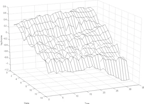
To analyze the income level of each state, we utilize the real per capita State Domestic Product (SDP) of 14 major states in 1970-2000.8 These 14 states account for 87.4 per cent of the population and 91.2 per cent of overall SDP, therefore, they are sufficient to represent the Indian economy. We adjust per capita income in terms of the 1980 levels, and denote it by . Figure 1 plots the series of the logs of per capita income less the state average, Eq. (1). It shows that the per capita income difference appears to increase gradually. In particular, the levels of lower income states tend to decline against the average as time moves to the recent period. Consequently, at a glance, the income differences across the states seem not to converge.
} {yit
8 The sample states are Maharashtra, Punjab, Haryana, Gujarat, Tamil Nadu, West Bengal, Karnataka, Kerala, Rajasthan, Andhra Pradesh, Madhya Pradesh, Uttar Pradesh, Orissa, and Bihar.
There is a serious problem in selecting the sample states. Because economic activities in northeastern states, economically small states and union territories are strongly affected by the central government, we exclude these states as previous studies did. See Kurian (1999) for details.
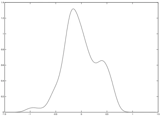
To investigate the distribution of these sequences, we estimate the nonparametric density for all states and sample periods. The results are shown in Figure 2. The per capita income distributes almost around the average, but is asymmetric. There is a bump in the upper tail. The lower tail is a bit longer than the upper tail.
However, a structural change may have taken place during the period. For instance, the Indian government began a partial economic liberalization from the mid-1980s, and then launched more comprehensive liberalization from 1991 in the aftermath of the balance of payment crisis.
Therefore, dividing the sample might change the results dramatically.
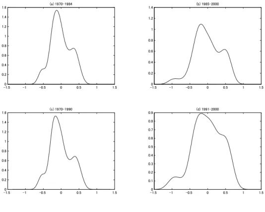
We first divide it into two sub-samples 1970-1984 and 1985-2000 in consideration of the beginning of economic liberalization in the mid-1980s. Figure 3a shows the density estimation in 1970-1984. It is nearly similar to that in Figure 2, and the peak is located around zero. On the other hand, Figure 3b represents the density estimation in 1985-2000; it has two bumps on both tails and a peak that leans into the lower tail. It looks like “twin peaks,” as Quah suggests regarding the income dispersion of the U.S. and OECD countries.
We then divide it into the periods 1970-1990 and 1991-2000. Figure 3c gives the density estimation of the sub-sample for 1970-1990. The shape does not seem different from that of Figure 2 or Figure 3a. In Figure 3d, however, the density for the 1991-2000 sample seems to have “triple peaks.” That is, it reveals three groups: high-, middle-, and low-income groups. As noted in Figure 1, the low-income group tends to be independently distributed in the recent period. Furthermore, the high-income group appears to be independently distributed against the other groups. These results are inconsistent with the convergence hypothesis.
4.2 Markov Transition Matrix
In place of the Barro regression, we first use an alternative method, the Markov transition matrix proposed by Quah (1993). The sample is the same as that in Figure 1, i.e., Eq. (1). Following previous studies, the number of states is chosen to be five, and the upper endpoint for each state is set so as to make the sample a uniform distribution. Table 1a shows the estimation of the Markov matrix for 1970-2000. The element in the matrix denotes the probability that an economy will move from state to . In this sample, the per capita income of each Indian state seems to be persistent, since the diagonal elements of the matrix are large. Further, the ergodic distribution, which denotes a long-run distribution, is scattered. Although there is a moderate likelihood of moving to an upper level, it appears to be a uniform distribution and there is no change in the income dispersion.
) , (i j j i
As noted in the last section, however, this feature may vary according to how the sub-samples are estimated. We first estimate Markov matrices for the periods 1970-1984 and 1985-2000. Table 1b presents the estimated matrix for the 1970-1984 sample. With the exception of the relatively small value of the (1,1) element, the matrix is not different from that of the 1970-2000 sample. Since its ergodic distribution is roughly similar, moreover, it is not reasonable to think that the per capita income tends to converge in this period. In the meanwhile, Table 1c shows an estimate of the matrix in the period 1985-2000. The (1,1) element is estimated to be higher than that in the last period, but the ergodic distribution is not different.
Next, we set the break point to be 1991, and estimate the Markov matrices. Table 1d reports the results for the period 1970-1990. Each element and the ergodic distribution are identical to those of Table 1b, so the income level does not seem to converge in this period. The matrix estimated in the period 1991-2000 is shown in Table 1e. The diagonal elements of this matrix are nearly all larger than those in other periods. Furthermore, the ergodic distribution leans (i.e., converges) toward the lowest level.
The results of the estimates of the sub-sample with the break points 1985 and 1991 suggest the following implications. Comparing the periods before liberalization (Table 1b and 1d) and after liberalization (Table 1c and 1e), any diagonal element of the former is smaller than that of the latter, except for the (5,5) element. Since, in Table 1b and 1d, the (1,1) elements are relatively small and the (1,2) elements are relatively large, in particular, lower income states tend to move toward higher income states before the economic liberalization.
Per capita income in our sample generally leans somewhat toward the lower tail, but the result of Table 1e, which reveals a strange ergodic distribution, may be due to the scarcity of data since the Markov matrices are estimated using the maximum likelihood estimator. Thus, they may be not robust to changing the upper endpoint or including additional samples. As proved by Barro and Sala-i-Martin (2004, pp. 50-51), furthermore, the dispersion of per capita income does not necessarily present a rejection of (unconditional) convergence. Thus, we will perform the second alternative method in order to check the robustness of the hypothesis that per capita income dispersion in Indian states does not converge.
4.3 SURADF Tests
Here, we utilize the SURADF test proposed by Breuer et al. (2002) to investigate whether or not per capita income is stationary and non-constant. According to Evans and Karras (1996), the income level of a state less the average income converges in a time-series sense if some conditions we noted above are satisfied. Breuer et al. (2002) show from Monte Carlo simulations that the SURADF test is superior to equation-by-equation ADF tests in terms of power. Phillips and Sul (2003) also perform the panel unit-root test assuming certain parametric relations, whereas SURADF has no need to include assumptions for such relations. Therefore, it is one of the most reliable methodologies for
testing the convergence hypothesis statistically.
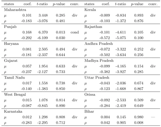
We specify the model to be Eq. (3). Table 2 shows the results of the estimation with a constant and a lagged difference. We arbitrarily choose p=1, but the lag length does not affect the results. The condition for unconditional convergence is to satisfy both µ=0 and ρ<0, but the results for all equations do not satisfy this condition. Only the equation for Punjab holds conditional convergence as required to satisfy µ≠0 and ρ<0. However, the estimation for Bihar has a significantly positive value for ρ, so the specification of this system may be doubtful.
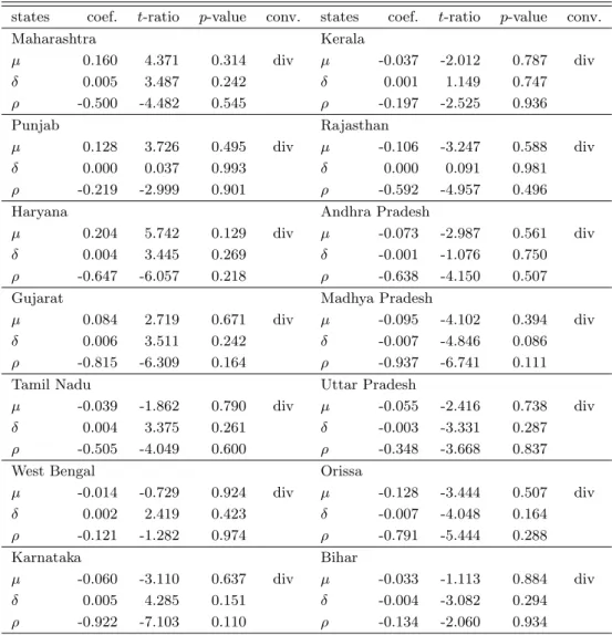
As noted by Greasley and Oxley (1997), if two sequences of income levels converge, the sequence of their difference should have no trend. Therefore, we need to investigate whether or not these equations have any trends and whether or not the results shown above change. We introduce a time trend into Eq. (3),
∑
,=
−
− + ∆ +
+ +
=
∆
p
s
t s t s t
t t x x
x
1
1 , 1 1 1 , 1 1 1 1
1 µ δ ρ ς ε
Μ (4)
∑
.=
−
− + ∆ +
+ +
=
∆
p
s
Nt s t N Ns t
N N N N
Nt t x x
x
1
, 1
, ς ε
ρ δ µ
The result of the estimation for Eq. (4) is shown in Table 3. The condition for unconditional convergence in this system is to satisfy µ=0, δ =0, and ρ<0, whereas that for conditional convergence is to satisfy ρ<0, and µ≠0 or δ≠0. In this case, no equations satisfy the conditions for either unconditional or conditional convergence.9
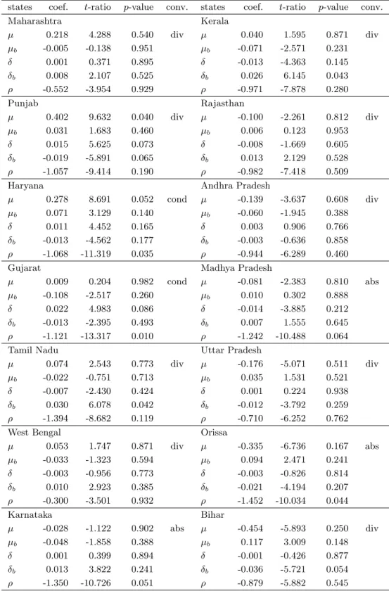
For U.S. regions, Carlino and Mills (1993) and Loewy and Papell (1996) consider a model with a structural break, and conclude that the hypothesis of conditional convergence is supported. To confirm the existence of a structural break in our data, we estimate Eq. (4) with an exogenous trend break. The model is
9 We also examine some popular univariate unit-root tests (DF-GLS, , , , and ), but the results are the same as with SURADF. So, our result is robust.
MZa MZt MSB MPT
∑
=−
− + ∆ +
+
−
>
+ +
>
+
=
∆
p
s
t s t s t
b b b b
b
t t T t t t t T x x
x
1
1 , 1 1 1
, 1 1 1
1 1
1
1 µ µ 1( ) δ δ 1( )( ) ρ ς ε ,
Μ (5)
∑
=−
− + ∆ +
+
−
>
+ +
>
+
=
∆
p
s
Nt s t N Ns t
N N b b bN N b bN N
Nt t T t t T t T x x
x
1
, 1
) ,
)(
( 1 )
(
1 δ δ ρ ς ε
µ
µ ,
where is the indicator function and is a fixed break point. In this case, each sequence converges unconditionally if all of the coefficient estimates of the deterministic trend are significantly different from zero and if
) (
1⋅ Tb
<0
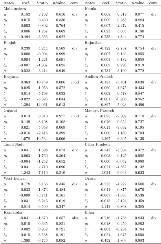
ρ , and converges conditionally if at least one of them is significant and if ρ<0. The estimation with a break at 1985 is presented in Table 4. According to this estimation, five of 14 sequences for per capita income are stationary, and three sequences do converge unconditionally (Madhya Pradesh, Orissa, and Karnataka) at the 10 percent significance level. However, at the 5 percent significance level, the number of stationary sequences falls to three, and that of unconditionally convergence to one. Next, we set the structural break at 1991, and present the results in Table 5. In this case, only one sequence (Karnataka) converges unconditionally and two sequences (Haryana and Gujarat) converge conditionally at the 10 percent significance level.
At the 5 percent level, all of the sequences except Haryana diverge. The coefficient estimate of the 1991 break in Haryana is significantly negative, so per capita income seems to deteriorate after economic liberalization.
Putting all this together, real per capita incomes across the Indian states generally tend to diverge. This tendency changes slightly if a structural break is considered, but more than half of the states still diverge.
5. Discussion
As concluded by most of the earlier papers on the Indian context, we reject the convergence
hypothesis, and find strong support for the hypothesis that income divergence among the Indian states has occurred since economic liberalization. Considering transition dynamics also gives us new insights. First, through the estimation of nonparametric density we find that the income dispersion of Indian states has triple peaks. In other words, Indian states are divided into high, middle and low income groups. Second, through a Markov transition matrix we find that lower income states tended to become higher income states before economic liberalization, whereas this possibility has decreased after economic liberalization.
The results estimated above are somewhat different from those of studies on other countries. On the estimations of Markov matrix, the ergodic distribution does not indicate convergence in either study, whereas the mobility of income level of Indian states is greater than that of other countries. To get a grasp of this fact, we find the mobility index introduced by Shorrocks (1978),
1 ) ) tr(
( −
= − n
Mp n P
P ,
where is a Markov matrix (n ) and denotes a trace of . The index takes a value from 0 to 1, and is greater as the factor moves more. Geweke et al. (1986) propose many indices of mobility. Since these do not vary in our samples, we utilize only the Shorrocks index. Now, let
be the estimated Markov matrix in Table 1a. The mobility index of is
P ×n
tr(P ) P
PIND PIND
(0.025).
300 . 0 ) (PIND = Mp
The standard error is in parentheses (for the estimation, see Schluter, 1998). We compare the indices before and after the economic liberalizations. Let PINDi (i=b,c,d,e) be the estimated Markov matrices in Table 1b-e The mobility indices of the matrices in 1970-1984 and 1985-2000 are
374 . 0 ) (PINDb =
Mp (0.039), Mp(PINDc )=0.245 (0.035), and those in 1970-1990 and 1991-2000 are
358 . 0 ) (PINDd =
Mp (0.032), Mp(PINDe )=0.204 (0.047).
After the economic liberalizations in 1985 and 1991, the indices clearly decline.
We next compare these estimates and those of other countries. Let and be the estimated Markov matrices of the U.S. (estimated by Quah, 1996b, Table 3) and Japan (Kawagoe, 1999, Table II.A), respectively. The mobility indices of these matrices are
PUS PJPN
(0.009), M (0.011).
160 . 0 ) (PUS =
Mp p(PJPN)=0.193
These indices are significantly different from that of our full-sample matrix, . The p-values, under the null hypothesis that the matrices are identical, are 0.001 and 0.000, respectively. This suggests that income mobility of Indian states is greater than that of regions in other (industrial) countries. Yet, this is not necessarily a desirable result because the per capita income is prone not only to increase but also to decrease. This high mobility of per capita income is one of the interesting features of Indian states. Moreover, the mobility index of the post-1991 liberalization matrix, , is closer to the indices of the U.S. and Japan (the p-values are 0.215 and 0.420, respectively). This may imply that the mobility of real per capita income tends to be more persistent after economic liberalization, or that a freer economy tends to have more persistent income dynamics.
PIND
e
PIND
The results from the SURADF tests also differ from previous papers that utilize panel unit-root tests. For instance, Holmes (2002) uses SURADF to investigate convergence across OECD countries, and concludes that some results support the hypothesis. Phillips and Sul (2003) use a unit-root test with certain parametric correlations for each equation to state that, for some groups, the convergence hypothesis may hold in the sample of Penn World Tables. On the contrary, our estimations on 14 Indian states suggest that few sequences of per capita income converge, and rather that almost all tend to diverge because they are non-stationary.
A question naturally arises from the facts noted above: Why does the real per capita
income of these states tend to diverge after economic liberalization? Many researchers offer answers, but they are still controversial. Physical or institutional infrastructure is a candidate. Aiyar (2001) examines the sequence of literacy rates in each state, and points out that the rates account for the difference of per capita income growth. More generally, Nagaraj et al. (1998) suggest that many forms of physical, economic, and social infrastructure affect the convergence across states. However, they do not state explicitly whether these factors have changed since the economic liberalization, and are critical toward the hypothesis of income dispersion. Actually, Sachs et al. (2002) investigate the impact of various factors on economic growth using data from the recent period, and reject the possibility.
The development of the financial system also causes little change in income disparity between the pre- and post-reform periods. Battacharya and Sivasubramanian (2003) regard M3 as a proxy for financial development, and investigate the long-run relationship between it and real GDP.
According to their results, these variables have a cointegration relation but show no structural break at 1991. Even if the model is estimated taking account of the break, the result does not vary. Their estimation uses aggregate rather than per capita output, but the result is interesting.
In addition, Cashin and Sahay (1996) carefully investigate the expansion of income dispersion, and support unconditional convergence. Their finding on the 1961-1991 data is that more grants from the central government flowed to poorer states, and that net migration had little impact on income convergence. They use pre-liberalization data, so their results may be influenced by the changes of the transfer of grants or migration.
Therefore, there is a discrepancy between these studies on the factors that generate income dispersion across the Indian states. Determining the reasons more accurately is a task for the future.
6. Concluding Remarks
In this paper, we used two alternative methods, i.e., Markov matrix estimations and SURADF tests, to investigate the convergence hypothesis of per capita income across 14 Indian states in 1970-2000.
The estimated Markov matrices suggest that, in the full sample period, the long-run distribution of per capita income scatters and does not vary, although it tends to rise slightly to a higher level. On the other hand, the estimation split into two sub-samples at break points at 1985 and 1991, when the government induced economic liberalization, implying that lower income states were able to rise in status before the economic liberalization, whereas they could not do so afterward. That is, in the recent period, low-income states continue to be poor and high-income states to be rich.
Furthermore, the results from the SURADF tests show that the sequences of per capita income are random walk processes, and so tend to diverge. This differs from the results of previous cross-country studies and U.S. regional studies, which confirm convergence between some sub-samples (countries or states). Our panel unit-root test rejects the convergence hypothesis, and the sequences have unit root. Hence, the sequences of per capita income across Indian states tend to diverge rather than converge.
Many recent studies using cross-country data investigate the convergence of per capita income under the time-series definition of Bernard and Durlauf (1996) or Evans and Karras (1996), and almost all partly support the hypothesis. Turning our eyes to the Indian economy, however, the departure from convergence clearly appears. To perform the hypothesis testing more rigorously, it may be necessary to utilize another methodology, e.g., a unit-root test with transitional dynamics,10 or to investigate domestic convergence in other developing countries.
10 See Lucke and Lutkepohl (2004). However, they show that standard unit-root tests are prone to reject the null hypothesis, so our conclusion would remain even when such a test is applied.
Data Appendix
State Domestic Product (SDP) represents income originating from within the geographical boundary of a state and the value added of goods and services within the state. Due to a lack of data on flow of factor income, they do not fully reflect income accruing to the residents of a state.
The estimation of SDP is conducted by respective state governments according to the concepts and methodology recommended by the Central Statistical Organization (CSO). Owing to differences in the source material used, data availability and extent of statistical development achieved, the estimates of various states are not strictly comparable. However, this data provides the only estimates available for a long time period and the effect of the accounting variations on comparisons is minor.
The sources of data are: (1) Estimates of State Domestic Product, CSO, Government of India, (2) EPW National Accounts Statistics in India 1950/51 to 1996/97, EPW Research Foundation, and (3) Economic Survey (2002-2003), Government of India.
References
Ahluwalia, M.S., 2000. Economic performance of states in post-reforms periods. Economic and Political Weekly, May 6, 1637-1648.
Aiyar, S., 2001. Growth theory and convergence across Indian states: a panel study, in: Callen, T., Reynolds, P., Towe, C. (Eds.), India at the Crossroads: Sustaining Growth and Reducing Poverty, IMF, 143-169.
Amemiya, T., 1985. Advanced Econometrics, Harvard University Press, Cambridge, Massachusetts.
Barro, R., Sala-i-Martin, X., 1991. Convergence across states and regions. Brookings Papers on Economic Activity 1, 107-158.
Barro, R., Sala-i-Martin, X., 1992. Convergence. Journal of Political Economy 100, 223-251.
Barro, R., Sala-i-Martin, X., 1995. Economic Growth. McGraw-Hill.
Barro, R., Sala-i-Martin, X., 2004. Economic Growth. Second Edition, MIT Press.
Baumol, W.J., 1986. Productivity growth, convergence, and welfare: what the long-run data show.
American Economic Review 76, 1072-1085.
Bernard, A.B., Durlauf, S.N., 1995. Convergence in international output. Journal of Applied Econometrics 10, 97-108.
Bernard, A.B., Durlauf, S.N., 1996. Interpreting tests of the convergence hypothesis. Journal of Econometrics 71, 161-173.
Bhattacharya, P.C., Sivasubramanian, M.N., 2003. Financial development and economic growth in India: 1970-1971 to 1998-1999. Applied Financial Economics 13, 905-909
Breuer, J.B., McNown, R., Wallace, M., 2002. Series-specific unit root tests with panel data. Oxford Bulletin of Economics and Statistics 64, 527-546.
Carlino, G.A., Mills, L.O., 1993. Are U.S. regional incomes converging? A time series analysis.
Journal of Monetary Economics 32, 335-346.
Cashin, P., Sahay, R., 1996. Internal migration, centre-state grants, and economic growth in the states of India. IMF Staff Papers 43, 123-171.
Das, S.K., Barua, A., 1996. Regional inequalities, economic growth and liberalization: a study of the Indian economy. Journal of Development Studies 32, 364-390.
Dasgupta, D., Maiti, P., Mukherjee, R., Sarkar, S., 2000. Growth and interstate disparities in India.
Economic and Political Weekly, July 1, 2413-2422.
De Long, J.B., 1988. Productivity growth, convergence, and welfare: comment. American Economic Review 78, 1138-1154.
Durlauf, S.N., Quah, D., 1999. The new empirics of economic growth, in: Taylor, J.B., Woodford, M.
(Eds.), Handbook of Macroeconomics, Vol. 1, North-Holland, Amsterdam, pp. 235-308.
Evans, P., Karras, G., 1996. Convergence revisited. Journal of Monetary Economics 37, 249-265.
Friedman, M., 1992. Do old fallacies ever die? Journal of Economic Literature 30, 2129-2132.
Geweke, J., Marshall, R.C., Zarkin, G.A., 1986. Mobility indices in continuous time Markov chains.
Econometrica 54, 1407-1423.
Ghosh, B., Marjit, S., Neogi, C., 1998. Economic growth and regional divergence in India: 1960 to 1995. Economic and Political Weekly, June 27-3, 1623-1630.
Greasley, D., Oxley, L., 1997. Time-series based tests of the convergence hypothesis: some positive results. Economics Letters 56, 143-147.
Holmes, M.J., 2002. Convergence in international output: evidence from panel data unit root tests.
Journal of Economic Integration 17, 826-838.
Im, K.S., Pesaran, M.H., Shin, Y., 2003. Testing for unit roots in heterogeneous panels. Journal of Econometrics 115, 53-74.
International Monetary Fund, 2004. World Economic Outlook, April 2004.
Islam, N., 1995. Growth empirics: a panel data approach. Quarterly Journal of Economics. 110, 1127-1170.
Johansen, S., 1988. Statistical analysis of cointegration vectors. Journal of Economic Dynamics and Control 12, 231-254.
Kakwani, N.C., 1967. The unbiasedness of Zellner’s seemingly unrelated regression equations estimators. Journal of the American Statistical Association 62, 141-142.
Kawagoe, M. 1999. Regional dynamics in Japan: a reexamination of Barro regressions. Journal of the Japanese and International Economies 13, 61-72.
Kurian, N.J., 1999. State government finances: a survey of recent trends. Economic and Political Weekly, May 8-14, 1115-1125.
Kurian, N.J., 2000. Widening regional disparities in India: some indicators. Economic and Political Weekly, February 12, 538-550.
Kwiatkowski, D., Phillips, P.C.B., Schmidt, P., Shin, Y., 1992. Testing the null hypothesis of stationarity against the alternative of a unit root. Journal of Econometrics 54, 159-178.
Loewy, M.B., Papell, D.H., 1996. Are U.S. regional incomes converging? Some further evidence.
Journal of Monetary Economics 38, 587-598.
Lucas, R.E., Jr., 1988. On the mechanics of economic growth. Journal of Monetary Economics 22, 3-42.
Lucke, B., Lutkepohl, H., 2004. On unit root tests in the presence of transitional growth. Economics Letters 84, 323-327.
Maddala, G.S., Wu, S., 1999. A comparative study of unit root tests with panel data and a new simple test. Oxford Bulletin of Economics and Statistics, Special Issue, 631-652.
Mankiw, N.G., Romer, D., Weil, D.N., 1992. A contribution to the empirics of economic growth.
Quarterly Journal of Economics 107, 407-437.
Marjit, S., Mitra, S., 1996. Convergence in regional growth rates: Indian research agenda. Economic and Political Weekly, August 17, 2239-2242.
Nagaraj, R., Varoudakis, A., Veganzones, M.A., 2000. Long-run growth trends and convergence across Indian states. Journal of International Development 12, 45-70.
Pagan, A., Ullah, A., 1999. Nonparametric Econometrics. Cambridge University Press.
Phillips, P.C.B., Sul, D., 2003. The elusive empirical shadow of growth convergence. Cowles Foundation Discussion Paper, No. 1398, Yale University.
Quah, D., 1993a. Galton’s fallacy and tests of the convergence hypothesis. Scandinavian Journal of Economics 95, 427-443.
Quah, D., 1993b. Empirical cross-section dynamics in economic growth. European Economic Review 37, 426-434.
Quah, D., 1996a. Regional convergence clusters across Europe. European Economic Review 40, 951-958.
Quah, D., 1996b. Empirics for economic growth and convergence. European Economic Review 40, 1353-1375.
Rao, M.G., Shand, R.T., Kalirajan, K.P., 1999. Convergence of incomes across Indian states: a divergent view. Economic and Political Weekly, March 27-April 2, 769-778.
Ric, S., Bhide, S., 2000. Sources of economic growth: regional dimension of reforms. Economic and Political Weekly, October 14, 3747-3757.
Romer, D., 1996. Advanced Macroeconomics. McGraw-Hill, New York.
Romer, D., 2001. Advanced Macroeconomics, Second Edition. McGraw-Hill, New York.
Sachs, J.D., Bajpai, N., Ramiah, A., 2002. Understanding regional economic growth in India. Asian Economic Papers 1, 32-62.
Schluter, C., 1998. Statistical inference with mobility indices. Economics Letters 59, 157-162.
Shorrocks, A., 1978. The measurement of mobility. Econometrica 46, 1013-1024.
Figure 1: Log per capita real income (3D plot)
Note: This graph plots log per capita real incomes of 14 Indian states during the period 1970-2000. The x-axis denotes time-horizon, y-axis states’ number, and z-axis log per capita real income.
Figure 2: Nonparametric density estimate: 1970-2000
Note: This figure shows the nonparametric density using the Rosenblatt-Parzen kernel density estimator with a Gaussian kernel. The bandwidth is chosen to ben−1/5σˆwhere n is the number of observations and ˆσ is the estimated standard error (see Pagan and Ullah, 1999). The sample period is 1970-2000.
Figure 3: Nonparametric density estimates: subsamples
Note: The sample periods are (a) 1970-1984, (b) 1985-2000, (c) 1970-1990, and (d) 1991- 2000.
Table 1: Transition matrices
(a) 1970-2000
Upper endpoint
Number -0.242 -0.122 0.040 0.340 infinity 84 0.762 0.214 0.024
84 0.286 0.583 0.131
85 0.165 0.682 0.153
83 0.133 0.807 0.060
84 0.036 0.964
Ergodic 0.194 0.162 0.157 0.181 0.306
(b) 1970-1984
Upper endpoint
Number -0.242 -0.122 0.040 0.340 infinity 29 0.586 0.379 0.035
41 0.342 0.512 0.146
54 0.185 0.685 0.130
40 0.175 0.750 0.075
32 0.031 0.969
Ergodic 0.160 0.194 0.183 0.136 0.326
(c) 1985-2000
Upper endpoint
Number -0.242 -0.122 0.040 0.340 infinity 52 0.885 0.096 0.019
39 0.205 0.667 0.128
29 0.138 0.655 0.207
41 0.098 0.854 0.049
49 0.041 0.959
Ergodic 0.188 0.106 0.125 0.265 0.316
(d) 1970-1990
Upper endpoint
Number -0.242 -0.122 0.040 0.340 infinity 45 0.556 0.400 0.044
66 0.333 0.561 0.106
68 0.162 0.706 0.132
51 0.177 0.765 0.059
50 0.020 0.980
Ergodic 0.145 0.194 0.167 0.125 0.369
(e) 1991-2000
Upper endpoint
Number -0.242 -0.122 0.040 0.340 infinity 36 1.000
15 0.067 0.667 0.267
14 0.143 0.714 0.143
30 0.067 0.867 0.067
31 0.065 0.936
Ergodic 1.000 0.000 0.000 0.000 0.000 Note: These tables report the estimated Markov transition matrices. The matrices are first order, time-stationary, and for five states. The upper endpoints are chosen to be uni- formly distributed in the data 1970-2000.
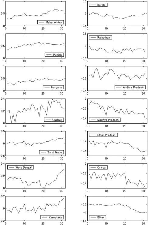
Figure 4: Log per capita real income (time-series plot)
"!
#
$%
&
' (*)+-, .
#
/10243506%+
&
78%9:;
&
<
<
70+
&
<
<
=<2
&
<#
&
<
&
<#
&
<
&
<#
&
<
A<9B.0
&
<#
&
<
CD)%
&
&
&
<
35)
Table 2: SURADF tests for convergence (without trend)
states coef. t-ratio p-value conv. states coef. t-ratio p-value conv.
Maharashtra Kerala
µ 0.101 3.448 0.285 div µ -0.009 -0.834 0.893 div
ρ -0.183 -3.076 0.481 ρ -0.103 -1.372 0.876
Punjab Rajasthan
µ 0.168 6.370 0.013 cond µ -0.101 -4.611 0.105 div
ρ -0.292 -6.109 0.030 ρ -0.572 -5.075 0.100
Haryana Andhra Pradesh
µ 0.081 2.505 0.494 div µ -0.072 -3.322 0.252 div
ρ -0.181 -2.337 0.644 ρ -0.502 -3.634 0.256
Gujarat Madhya Pradesh
µ 0.057 1.954 0.633 div µ -0.099 -4.165 0.154 div
ρ -0.237 -2.127 0.733 ρ -0.382 -3.927 0.285
Tamil Nadu Uttar Pradesh
µ 0.017 1.558 0.738 div µ -0.043 -2.036 0.674 div
ρ -0.140 -1.383 0.850 ρ -0.123 -1.668 0.867
West Bengal Orissa
µ 0.015 1.078 0.814 div µ -0.092 -2.533 0.509 div
ρ -0.087 -0.845 0.890 ρ -0.284 -2.419 0.649
Karnataka Bihar
µ 0.012 1.298 0.808 div µ 0.004 0.145 0.980 —
ρ -0.283 -2.295 0.712 ρ 0.042 0.905 0.008
Note: This table reports the results from SURADF proposed by Breueret al. (2002). The data is a balanced panel withN= 14 andT = 31. Each equation includes a constant and one lagged first defference, but the coefficient estimates for lagged differences are not reported.p-values are obtained by the Monte Carlo simulations with 5,000 iterations. “Conv.” denotes whether or not the log of real per capita income converges at the 10 percent significance level, and abs, cond, and div denote unconditional convergence, conditional convergence, and divergence, respectively.