Prediction of Solvation Free Energy of Proteins: Molecular Dynamics Simulation and QSPR Model Approach

(1)

Molecular Dynamics Simulation and QSPR Model Approach

Sri R. Natasia

^a,b

, Hiroaki Saito

^a

, Taku Mizukami

^c

, Kazutomo Kawaguchi

^a

, Hidemi Nagao

^a

a

Institute of Science and Engineering, Kanazawa University, Kakuma, Kanazawa 920-1192 Japan,

b

Faculty of Mathematics and Natural Sciences, Institut Teknologi Bandung, Jl. Ganesha 10, Bandung 40132 Indonesia,

c

School of Material Science, Japan Advanced Institute of Science and Technology, Nomi, Ishikawa 923-1292 Japan,

E-mail: [email protected], [email protected]

Abstract. Solvation free energy has valuable role as represents the desolvation cost of a molecu- lar binding interaction, which is very important in a variety of chemical and biological processes.

Therefore, many computational methods have been explored to predict this value. In this study, we attempted to find the correlation between experimental and calculated value of solvation free energy of proteins, containing organic molecules, by using quantitative structure property relation- ship (QSPR) model. To obtained a comparable value of solvation free energy which will be used as reference in QSPR model, we adopted energy representation (ER) method. And as this method works through molecular dynamic (MD) simulation, we then performed the MD simulation prior to the calculation by ER method. The results showed that the predicted solvation free energies were quite close to calculated values by ER method. We also found that the values of solvation free energy, both in MD simulation and ER method, were well correlated to solvent accessible surface area of hydrophobic portion.

Keywords: solvation free energy, organic molecules, proteins, molecular dynamics, ER method, QSPR model

1 Introduction

Solvation free energy is one of the most important physical quantity to describe thermal system of a solution. It has valuable role as represents the desolvation cost of a molecular binding interaction [1], which is very important in a variety of chemical and biological processes. For instances, in drug discovery and in analysis of protein folding and binding. Therefore, many computational methods have been explored to predict this value.

In recent years, quantitative structure-property relationship (QSPR) model has been widely used in chemical physics area to predict some physical quantities of organic materials. QSPR model is well known for its simplicity yet has the ability to provide a promising result. This approach attempts to relate the structure-derived property of a chemicals to its biological or physicochemical activity. One of the most fundamental and common modeling method in QSPR is multiple linear regression, which is favored for its simplicity and ease of interpretation [2].

In construction QSPR model of protein, a reliable data of solvation free energy is strongly needed.

However, due to limitation in experimental measurements, solvation free energy of protein is still

rare even unavailable. Hence, to provide such value, we adopted energy representation [3] (ER)

method which has been successfully applied for many biological systems [4].

(2)

Here, firstly we employ ER method to calculate solvation free energy of 50 organic molecules containing diverse organic functions in explicit water solvent. As the calculation using this method is obtained in combination with molecular dynamics (MD) simulation [5], we carry out the MD simulation of each molecule prior to the calculation of this value. In order to confirm the validity of this method, we then compare the results to experimental data. Further, we compute solvation free energy of proteins and construct the QSPR model with utilizing MD simulation.

2 Materials

We calculated solvation free energies of 50 organic molecules containing diverse organic functions;

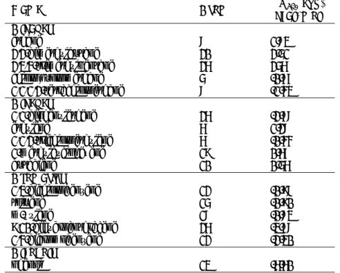
alkanes, alkenes, aromatics, alcohols, aldehydes, ketones, amines, ethers, esters, and others. The number of atoms is vary from 5 to 40. We retrieved the coordinate files of these molecules in mol2 format from reference [6]. The 50 organic molecules are listed in Table 1 below.

Table 1: The 50 organic molecules, number of atom and experimental value of ∆G

sol

Name Atom ∆G

sol

exp.

(kcal/mol) Alkanes

ethane 8 1.83

2,2-dimethylbutane 20 2.51

2,3,4-trimethylpentane 26 256

chlorofluoromethane 5 -0.77

1,1,1,2-tetrachloroethane 8 -1.43

Alkenes

1,1-diphenylethene 26 -2.78

ethylene 6 1.28

1,1,2-trichloroethylene 6 -0.44

1-methylcyclohexene 19 0.67

butadiene 10 0.56

Aromatics

1,3-dichlorobenzene 12 -0.98

toluene 15 -0.90

m-xylene 18 -0.83

9,10-dihydroanthracene 26 -3.78

1,4-dibromobenzene 12 -2.30

Alcohols

phenol 13 -6.60

(3)

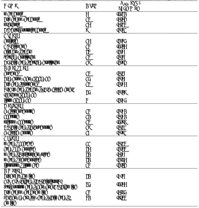
Table 1: The 50 organic molecules, number of atom and experimental value of ∆G

sol

(continued)

Name Atom ∆G

sol

exp.

(kcal/mol)

methanol 6 -5.10

2-methoxyethanol 13 -6.62

p-cresol 16 -6.13

2,2,2-trifluoroethanol 9 -4.31

Ethers

anisole 16 -2.45

1,4-dioxane 14 -5.06

diphenylether 23 -2.87

tetrahydrofuran 13 -3.47

2,5-dimethyltetrahydrofuran 19 -2.92

Aldehydes

butanal 13 -3.18

2-hydroxybenzaldehyde 15 -4.68

2-methylpropanal 13 -2.86

4-(1-methylethenyl)-1-cyclohexene-1 25 -4.09 -carboxaldehyde

formaldehyde 4 -2.75

Ketones

cyclopentanone 14 -4.70

acetone 10 -3.80

nitroxyacetone 13 -5.99

3,3-dimethyl-2-butanone 19 -3.11

cyclohexanone 17 -4.91

Esters

methyl acetate 11 -3.13

ethyl hexanoate 26 -2.23

methyl-4-nitrobenzoate 20 -6.88

methyl pentanoate 20 -2.56

isopropyl formate 14 -2.02

Amines

2-naphtylamine 20 -7.47

1-N,1-N-diethyl-2,6-dinitro-4-

(trifluoromethyl)benzene-1,3-diamine 35 -5.66

2-methoxyethanamine 14 -6.55

(2-benzhydryloxyethyl)-dimethyl- amine

40 -9.34

(4)

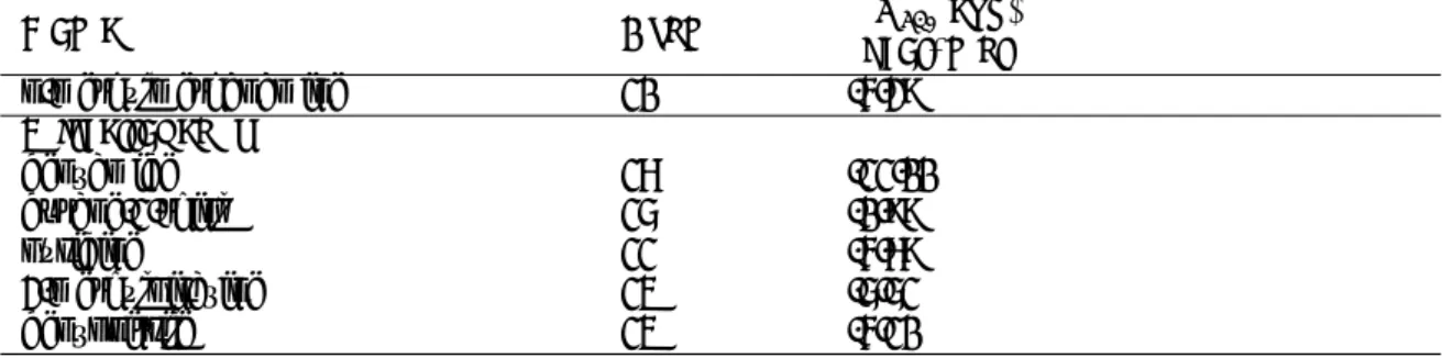
Table 1: The 50 organic molecules, number of atom and experimental value of ∆G

sol

(continued)

Name Atom ∆G

sol

exp.

(kcal/mol)

n-methylmethanamine 10 -4.29

Miscellaneous

benzamide 16 -11.00

butane-1-thiol 15 -0.99

pyridine 11 -4.69

2-methylpirazine 13 -5.51

benzonitrile 13 -4.10

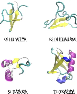
In construction of QSPR model of protein, we used 4 small and neutral charge proteins. These proteins were leginsulin, cysteine-rich module 3 from integrin beta-2 (the name is shortened as cysteine-rich in this paper), crambin, and ubiquitin. The initial structures were taken from X-ray diffraction and NMR solution from Protein Data Bank. The secondary structure of these proteins in ribbon representation using visual molecular dynamics (VMD) tools are shown in Figure 1. The protein data bank (PDB) ID, the number of residues and atoms are listed in Table 2.

3 Methods

3.1 MD Simulation

In MD simulations for organic molecule, the force field parameters and partial charge for each atom were assigned by antechamber [7] program of Amber tools in which general atom force field (GAFF) [8] and AM1-BCC [9, 10] were utilized. After generating Amber topology and coordinate files, these two files were converted to Gromacs topology and coordinate files using acpype [11]

conversion script. These organic molecules were then solvated in a simulation box of 32˚ A × 32˚ A

× 32˚ A which consists of 1000 water molecules using Gromacs utilities. The simulations were performed for 100 ps and sampled every 10 fs for solution system. Meanwhile, for pure solvent and isolated solute systems, the simulations were conducted for 10 ps and 10 ns and sampled every 200 fs.

Meanwhile, for protein system, we carried out MD simulations for 20-30 ns to obtain the equilibrium state of the system. The proteins were placed at the center of simulation box with the distance at least 12˚ A from the box edge. The box was then filled with water molecules to set the density of the system near to 1 g/cm

³

. The protein simulations were performed with AMBER99SB [12]

force field.

All MD simulations, for both organic molecules and proteins, were performed by Gromacs 4.6.5 program package. The conditions were generated through NPT ensemble at 300 K and 1 bar using Nose-Hoover thermostat and Parinello-Rahman barostat with time constant of 1 ps [13, 14]. The Lennard-Jones potential was applied for intermolecular interaction with cutoff length of 13.5 ˚ A.

To handle electrostatic interaction, particle-mesh Ewald (PME) [15] with interpolation order of 6

was used. TIP3P water model [16] were adopted for water molecules. And the simulations were

run with time step for integration of 2 fs.

(5)

(a) Leginsulin (b) Cysteine-rich

(c) Crambin (d) Ubiquitin

Figure 1: Various initial structure of proteins were taken from the original PDB file

Table 2: The protein data bank ID, the number of residues and atoms of 4 proteins [17–20].

Protein PDB ID Residue Atom

Leginsulin 1ju8 37 524

Cysteine-rich 1l3y 41 557

Crambin 1crn 46 642

Ubiquitin 1ubq 76 1231

3.2 Energy Representation

In energy representation (ER) method, solvation free energy can be represented as a functional of energy distribution functions ρ

^e

(ε) and ρ

^e₀

(ε) and the correlation matrix χ

^e₀

(ε, η) [4]. The energy distribution ρ

^e

(ε) is given by

ρ

^e

(ε) = h X

i

δ(v(ψ, x

i

) − ε)i (1)

where ψ is the solute coordinate, x

i

refers to the coordinate of the i -th solvent molecule, v is the potential function for the solute-solvent pair interaction, the summation is taken over all the solvent molecules, and h...i is the ensemble average.

The calculation using ER method is obtained in combination with MD simulation. Therefore, to get

the energy distribution functions and correlation matrix, we performed two kinds of MD simulation

prior to the calculation of solvation free energy for each organic material. These simulations are

solution system ρ

^e

(ε) and the pure solvent system ρ

^e₀

(ε). The solution system is the system in which

the interaction presents between the solute and the solvent molecule under the solute-solvent pair

interaction energy v of interest at full coupling. While the reference solvent system refers to the

system in which no interaction physically present between the solute and the solvent molecule [4].

(6)

0 0.5 1 1.5 2 2.5 3 3.5 4

0 5 10 15 20

RMSD (Å)

Time (ns)

Cysteine−Rich Leginsulin Crambin Ubiquitin

Figure 2: Root mean square displacement (RMSD) profiles of the four proteins

The energy distribution function ρ

^e₀

(ε) and correlation matrix χ

^e₀

(ε, η) are constructed by placing the solute into the pure solvent as a test particle.

In MD simulation of solution system for protein, the protein conformations were taken from the stable state of the 20 ns equilibration MD. From the last 10 ns simulation, the structure of protein was sampled every 200 ps, leading to 50 samplings of protein structure. For each structure, the MD simulation was performed in which the protein was in fixed condition. The simulation were run for 1 ns and was kept every 10 fs, yielding 100 k sampling data for the calculation of ρ

^e

(ε).

The next is the reference solvent system, which was used for the calculation of ρ

^e₀

(ε) and χ

^e₀

(ε, η).

The simulation was carried out for 1 ns and the snapshot was kept every 1 ps, leading to 1 k sampling data. The protein with random positions, yet same conformation as that in the solution system, were then inserted to the center of reference solvent system. The number of insertion sampling was 1000, hence we had 1000 k sampling data for the calculation of ρ

^e₀

(ε) and χ

^e₀

(ε, η).

The number of water molecule in both of simulation was equal to that in the prior equilibrium MD. These simulations were also conducted in NPT configuration.

3.3 QSPR Model

In construction of QSPR model, we adopted linear regression equation from Duffy and Jorgensen model [21]:

∆G

sol

= β < E

elec

> +α < E

vdW

> +γ < SASA > + (2) where E

elec

is the electrostatic (Coulomb) energy between solute and solvent molecule. E

vdW

represents the van der Waals (Lennard-Jones) interaction energy of solute-solvent. While SASA refers to solvent-accessible surface area of the solute by solvent molecule. The correlation coefficient β , α and γ are obtained from the covariance matrix among the MD simulation-derived descriptors and the reference solvation free energies, and is defined by:

cov ( y, x

_j

) =

k

X

m=1

b

_m

.cov ( x

_m

, x

_j

) j, m = 1 , ..., k (3)

(7)

where y is the reference solvation free energy, x the MD simulation-derived descriptors, k the number of descriptors, and b

_m

refers to correlation coefficient of each descriptor ( β , α and γ ). The covariance matrix is governed by the following equation:

cov(x, y) = P

n

i=1

(x

i

− x)(y ¯

i

− y) ¯

(n − 1) (4)

where x and y are the observed variables, can be the reference solvation free energy–descriptor or descriptor–descriptor. The index of i refers to the i-th data, while the bar signs refer to mean value of each observed variable. Then, the remaining becomes

= ¯ Y − X

m=1

b

m

x ¯

m

(5)

where ¯ Y is the mean value of the reference solvation free energy.

We also modified the equation 2 to asses the contribution of hydrophobic and hydrophilic properties of organic material. To do so, the SASA area was then divided into 2 parts, the areas of hydrophilic and hydrophobic portions of SASA (SASA

philic

and SASA

phobic

). The modified of equation 2 is shown below:

∆G

sol

= β < E

elec

> +α < E

vdW

> +γ

1

< SASA

phobic

> +γ

2

< SASA

philic

> + (6) The average values of all descriptors in equation (2) and (6) were calculated using g energy and g sas functions in Gromacs. The solvent probe radius of 1.4 ˚ A was defined in calculation of SASA by g sas function.

4 Results and Discussion

4.1 MD Simulation of Proteins

We calculated the root mean square displacement (RMSD) of backbone atoms of the four proteins to examine the stability of the systems during MD simulations. The RMSD curves are illustrated in Figure 2. These curves show that the three proteins reached the equilibrium state after about 10 ns simulation. Meanwhile, the RMSD profile of Cysteine-rich increased after 10 ns. Thus, to further see the dynamics of the system, the MD simulation was extended to 30 ns for this protein.

Later,we found that it was fully equilibrated after about 15 ns simulation. The average of RMSD of all protein systems at stable state were 0.58-3.22 ˚ A, indicating that overall dynamics structures were close to the native structures without large structural changes.

4.2 Solvation Free Energy by ER Method

The calculated solvation free energies of 50 organic molecules and the corresponding experimental data from reference [6] are shown in Figure 3.(a). We found that these values were in good agreement with the experimental data with the average of difference was about 2.09 kcal/mol.

We also investigated the solvation free energy with respect to the surface properties area of organic

molecules. Figure 3 (b) displays the solvation free energy and the value of whole SASA. From this

figure, we could tell that these two values do not correlate well for all organic molecules. Hence,

we further analyzed the surface area into SASA

phobic

and SASA

philic

as shown in Figure 3 (c) and

(d). Based on these figures, SASA

phobic

has positive correlation towards the solvation free energy,

(8)

−12 −10 −8 −6 −4 −2 0 2 4 6 8

−12

−10

−8

−6

−4

−2 0 2 4 6 8

Experimental solvation free energy (kcal/mol)

Calculatedsolvationfreeenergy(kcal/mol)

alcohols esters alkenes alkanes amines ketones aldehydes ethers aromatics miscellaneous Organic function:

(a)

0 100 200 300 400 500

−8

−6

−4

−2 0 2 4

SASA (˚A²)

(b)

0 100 200 300 400 500

−8

−6

−4

−2 0 2 4

Hydrophobic area (˚A²)

(c)

0 50 100 150 200 250 300

−8

−6

−4

−2 0 2 4

Hydrophilic area (˚A²)

(d)

Figure 3: The experimental vs calculated values of solvation free energy of organic molecules by ER method (a) and the surface properties area of the molecules (b), (c), (d)

denoted by the correlation coefficient r of 0.29. Whereas SASA

philic

shows weak correlation in which r = 0.11. It means SASA

phobic

has more contribution to the solvation free energy of organic molecules. In addition, we observed that almost all of the used molecules consisting of more hydrophobic than hydrophilic atom. And these figures also indicated that more hydrophobic areas of the molecules can be accessed by water solvent than the hydrophilic does.

On the other hand, for the calculation of solvation free energies of proteins, the results are shown in Figure 4 (a) as the protein size (see Table 3 for the actual values). According to these results, the solvation free energies vary depend on the number of atom on the system. Also, the current results of solvation free energies are negative, showing that the proteins can stably exist in pure water solvent. The examined surface properties of the four proteins are illustrated in Figure 4 (b) (the calculated values are listed in Table 3). This figure shows the larger the protein, the possibility of the solvent molecules to access the area is also increase. Especially, globular protein like ubiquitin which has many hydrophilic residues on the surfaces in contact with water, leading to the high value of SASA

philic

. In contrast, despite crambin also a globular protein, it is more known as

”inside out” globular protein in which containing more hydrophobic residues [22]. Therefore, this

protein is insoluble in water solvent indicated by the low value of SASA

philic

and the solvation free

energy.

(9)

−900

−800

−700

−600

−500

−400

−300

−200

−100 0

Leginsulin Cysteine−rich Crambin Ubiquitin

Solvation Free Energy (kcal/mol)

solvation free energy

(a)

0 1000 2000 3000 4000 5000 6000

SASA (Å2)

SASA: hydrophobic SASA: hydrophilic SASA

(b)

Figure 4: (a) Solvation free energies of the four proteins; and (b) The average of solvent accessible surface areas (SASA) of the four proteins; the green line: whole SASA, the red line: the SASA of hydrophilic portion (SASA

philic

), the blue line: the SASA of hydrophobic portion (SASA

_phobic

).

Table 3: Solvation free energies by ER method, the whole portion of solvent accessible surface area (SASA), the SASA of hydrophilic portion (SASA

philic

), and the SASA of hydrophobic portion (SASA

phobic

) of the four proteins.

Protein

Solvation

SASA SASA

philic

SASA

phobic

free energy

(kcal/mol) (˚ A

²

) (˚ A

²

) (˚ A

²

)

Leginsulin -378 2234 1190 1044

Cysteine-rich -528 2336 1164 1172

Crambin -208 2562 1137 1425

Ubiquitin -848 4210 2188 2022

4.3 Solvation Free Energy by QSPR Model

After performing the MD simulations and the solvation free energy calculation, we constructed the QSPR model using the MD simulation-derived descriptors from all organic molecules and proteins.

Based on the equations 2 and 6, we got the following model: -

∆G

sol

= 0.1616 < E

elec

> +0.3567 < E

vdW

> +0.1968 < SASA > −24.2945 (7)

∆ G

_sol

=0 . 1131 < E

elec

> +0 . 0085 < E

vdW

> +0 . 0679 < SASA

phobic

>

+ 0.0003 < SASA

philic

> −9.5278 (8)

which gave the squared correlation coefficient (R

²

) = 0.998 and mean square error (MSE) = 35.802, for the equation 7. Meanwhile, for the model which constructed by equation 8, the R

²

=0.994 and MSE = 144.477. These results indicated that our model which governed by equation 8 was quite good compare to Duffy and Jorgensen model. Moreover, the high values of R

²

in both of models suggest that the regression lines were well fitted to approximate the values of solvation free energy.

The predicted solvation free energies of organic molecules and four proteins are shown in Figure 5

(a),(c) and (b),(d), for the equation 7 and 8, respectively.

(10)

We also calculated the averages of difference of these two models toward the calculated value of solvation free energies of proteins and the experimetal data of organic molecules. For the proteins, these values were 7.88 and 34.61 kcal/mol, for the model by equation 7 and 8, respectively. And for the organic molecules, the averages of difference of these two models were 3.74 and 4.69 kcal/mol, respectively.

Additionally, in our model, we found that the SASA

phobic

has more significant contribution than the SASA

philic

, refers to the value of coefficient correlation in the equation 8. This positive correlation has also been presented in previous result by ER method. Moreover, the weak correlation between SASA

philic

and the solvation free energy as described in previous section also been made clear by value of coefficient correlation in our model. These results was supported by the finding of more hydrophobic atoms than hydrophilic in almost all organic molecules and proteins.

−10 −5 0 5 10

−10

−5 0 5 10

Predicted solvation free energy (kcal/mol)

alcohols esters alkenes alkanes amines ketones aldehydes ethers aromatics miscellaneous Organic function

(a)

−15 −10 −5 0 5

−15

−10

−5 0 5

Predicted solvation free energy (kcal/mol)

alcohols esters alkenes alkanes amines ketones aldehydes ethers aromatics miscellaneous Organic function

(b)

−800

−700

−600

−500

−400

−300

−200

Solvation free energy (kcal/mol)

ER method QSPR model equation 7

(c)

−800

−700

−600

−500

−400

−300

−200

Solvation free energy (kcal/mol)

ER method QSPR model equation 8

(d)

Figure 5: The QSPR model which governed by equation 7 (a),(c) and equation 8 (b),(d)

5 Conclusions

We carried out MD simulations of 4 small and neutral charge proteins, also 50 organic molecules containing diverse organic functions, to calculate solvation free energy of these organic materials.

We also constructed the QSPR model, which utilizing MD simulation, to investigate the correlation

(11)

to the experimental data and to the calculated results of ER method. However, due to limitation of experimental data of proteins, the comparison of solvation free energy could not be done. Thus, we compared the results of our model to the calculated values by ER method. The comparison indicated that the predicted values of protein were quite close to the calculated values by ER method. We also found that the solvation free energies of our organic materials, both in MD simulation and QSPR model, were well correlated with SASA

phobic

.

Acknowledgment

Some computations in this study were performed using computational resources at Research Center for Computational Science, Okazaki, Japan and Japan Advanced Institute of Science and Tech- nology (JAIST). This works was (partially) supported by a Grant-in-Aid for Scientific Research on Innovation Areas ”Chemical Biology of Natural Products” from The Ministry of Education, Culture, Sports, Science, and Technology, Japan.

References

[1] V. N. Viswanadgan, et. al (1999). Prediction of Solvation Free Energies of Small Organic Molecules: Additive-Constitutive Models Based on Molecular Fingerprints and Atomic Con- stants. J. Chem. Inf. Comput. Sci., 39, 405 – 412.

[2] M. Dehmer, et. al (2012). Statistical Modelling of Molecular Descriptors in QSAR/QSPR.

Wiley – VCH, Weinheim.

[3] N. Matubayashi and M. Nakahara (2000). Theory of solutions in the energetic representation.

I. Formulation. J. Chem. Phys., 113, 6070 – 6081.

[4] H.Saito, et. al. (2010). Hydration Property of Globular Proteins: an Analysis of Solvation Free Energy by Energy Representation Method. Chem. Phys. Letters, 497, 218 – 222.

[5] Y. Karino, et. al. (2010). End-Point Calculation of Solvation Free Energy of Amino-Acid Analogs by Molecular Theories of Solution. Chem. Phys. Letters, 496, 351 – 355.

[6] D. L. Mobley, et. al. (2009). Small Molecule Hydration Free Energies in Explicit Solvent: an Extensive Test of Fixed-Chrge Atomistic Simulations. J. Phys. Chem. B, 5(2), 350 – 358.

[7] J. Wang, et. al. (2006). Automatic Atom Type and Bond Type Perception in Molecular Mechanical Calculations. J. Mol. Graph. Mod. , 25 , 247 – 260.

[8] J. Wang, et. al. (2004). Development and Testing of a General AMBER Force Field. J. Comp.

Chem., 25, 1157 – 1174.

[9] A. Jakalian, et. al. (2000). Fast, Efficient Generation of High-Quality Atomic Charges. AM1- BCC Model: I. Method. J. Comp. Chem., 21(2), 132 – 146.

[10] A. Jakalian, et. al. (2002). Fast, Efficient Generation of High-Quality Atomic Charges. AM1- BCC Model: I. Parameterization and Validation.J. Comp. Chem., 23(16), 1623 – 1641.

[11] A. W. Sousa da Silva and W. F. Vranken. (2012). ACPYPE - AnteChamber PYthon Parser

interfacE. BMC Research Notes, 5, 367.

(12)

[12] V. Hornak, et. al (2006). Comparison of Multiple Amber Force Fields and Development of Improved Protein Backbone Parameters. Proteins , 65 , 712 – 725.

[13] M. E. Tuckerman, et. al (2001). Non Hamiltonian Molecular Dynamics: Generalizing Hamil- tonian Phase Space Principles to Non-Hamiltonian Systems. J. Chem. Phys., 115(4), 1678 – 1702.

[14] M. Parrinello and A. Rahman. (1980). Crystal Structure and Pair Potentials: a Molecular Dynamics Study. Phys. Rev. Lett., 45, 1196.

[15] T. Darden, et. al. (1993). Particle Mesh Ewald-an N.Log(N) Method for Ewald Sums in Large System. J. Chem. Phys., 98, 10089 – 10092.

[16] W. L. Jorgensen, et. al. (1983). Comparison of Simple Potential Functions for Simulating Liquid Water. J. Chem. Phys., 79(2), 926 – 935.

[17] T. Yamazaki, et. al. (2003). A Possible Physiological Function and the Tertiary Structure of a 4-kDa Peptide in Legumes. Eur. J. Biochem. , 270 , 1269 – 1276.

[18] N. Beglova, et. al. (2002). Cysteine-rich Module Structure Reveals a Fulcrum for Integrin Rearrangement Upon Activation. Nat. Struct. Biol., 9, 282 – 287.

[19] M. M. Teeter. (1984). Water Structure of a Hydrophobic Protein at Atomic Resolution: Pen- tagon Rings of Water Molecules in Crystals of Crambin. Proc. Natl. Acad. Sci. Usa., 81, 6014 – 6018.

[20] S. Vijay-Kumar. (1987). Structure of Ubiquitin Refined at 1.8 A Resoulution. J. Mol. Biol., 194, 531 – 544.

[21] E. M. Duffy and W. L. Jorgensen. (2000). Prediction of Properties from Simulations: Free Energies of Solvation in Hexadecane, Octanol, and Water. J. Am. Chem. Soc., 122, 2878 – 2888.