ガイダンス: 経済学とは
•
経済学のとは
①稀少の資源を有効的利用する方法を探す学問。
②現実に起きている経済現象を分析する理論と方法。
③人々を幸せさせる方法を探す学問。
GDP総額
1人当りGDP= ― ― ― ― ―
総人口
Enjoyment (享受)
幸せ公式:
Happiness=
---Desire (欲望)
方法1:経済パイ
(Pie)の拡大
—享受の拡大—GDP増大—経済成長、等
方法
2:経済パイの不変
--欲望の抑制--節約--所得の平等分配
方法
3:人口の抑制:1人当りGDP=GDP総額/人口
等々。
第2章 経済学の
10大原理
原理1:人々はトレードオフに直面する
原理2: あなたは何かを得るために放棄したのものコスト
(機会費用)
原理3: 理性ある国民はマージンで考えます
原理4: 人々は誘因に応じる
原理5: 貿易は皆の生活を向上させる
原理6: 市場は常に経済活動を動く早道
原理7: 政府は市場のもたらす成果を改善できることもある
原理8: 一 国の生活水準は、財・サービスの生産能力に
依存する
原理9: 政府が紙幣を印刷し過ぎると、価格が上昇する
原理10: 社会はインフレーションと失業の短期的トレードオ
フに直面している(例:フィリップス曲線)
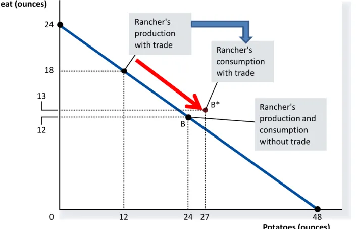
第3章 貿易と生産・消費の拡大
Figure 2 How Trade Expands the Set of Consumption Opportunities
Copyright © 2004 South-Western Potatoes (ounces) 12 24 13 27 B 0 Meat (ounces)
(b) The Rancher s Production and Consumption’
牛飼の場合は 48 24 12 18 B* Rancher's consumption with trade Rancher's production with trade Rancher's production and consumption without trade
第3章 比較優位
• 生産費用の差の測り方法は二つある
1. 1単位当たり製品を生産するために必要な時間
製品の生産量
労働生産性=
労働時間(労働者人数)
2
. 1つの製品を生産するためにやめた別の製品
の機会費用(図で説明)
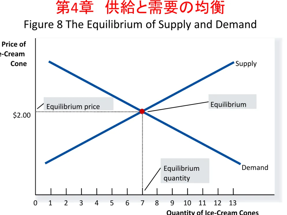
第
4章 需要と供給
均
衡
価
格
第
4章 供給と需要の均衡
Figure 8 The Equilibrium of Supply and Demand
Price of
Ice-Cream
Cone
0
1
2
3
4
5
6
7
8
9 10 11 12
Quantity of Ice-Cream Cones
13
Equilibrium
quantity
Equilibrium price
Equilibrium
Supply
Demand
$2.00
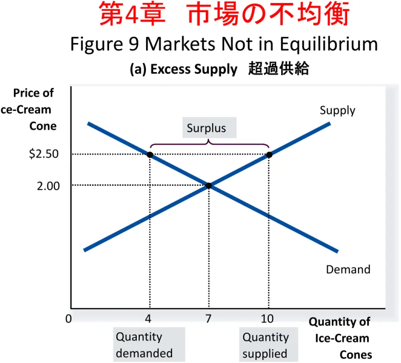
第
4章 市場の不均衡
Figure 9 Markets Not in Equilibrium
Price of
Ice-Cream
Cone
0
Supply
Demand
(a) Excess Supply 超過供給
Quantity
demanded
Quantity
supplied
Surplus
Quantity of
Ice-Cream
Cones
4
$2.50
10
2.00
7
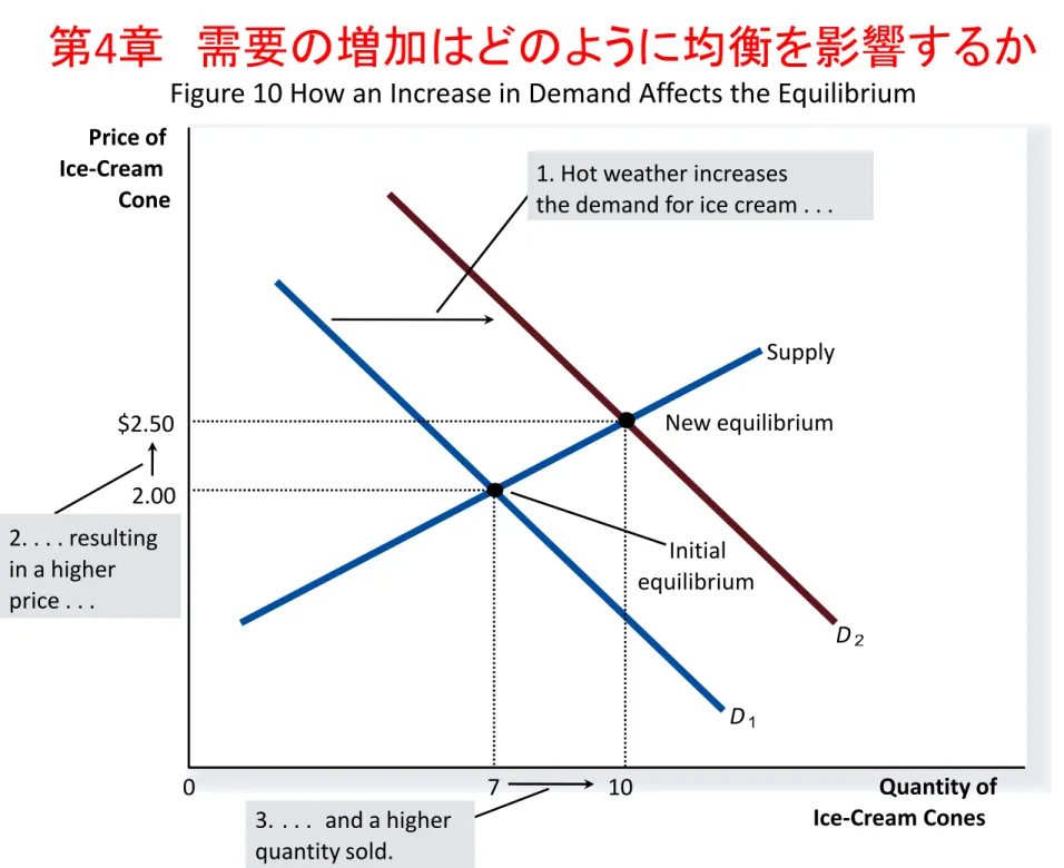
Price of Ice-Cream Cone 0 Quantity of Ice-Cream Cones Supply Initial equilibrium D D 3. . . . and a higher quantity sold. 2. . . . resulting in a higher price . . .
1. Hot weather increases the demand for ice cream . . .
2.00 7 New equilibrium $2.50 10
第
4章 需要の増加はどのように均衡を影響するか
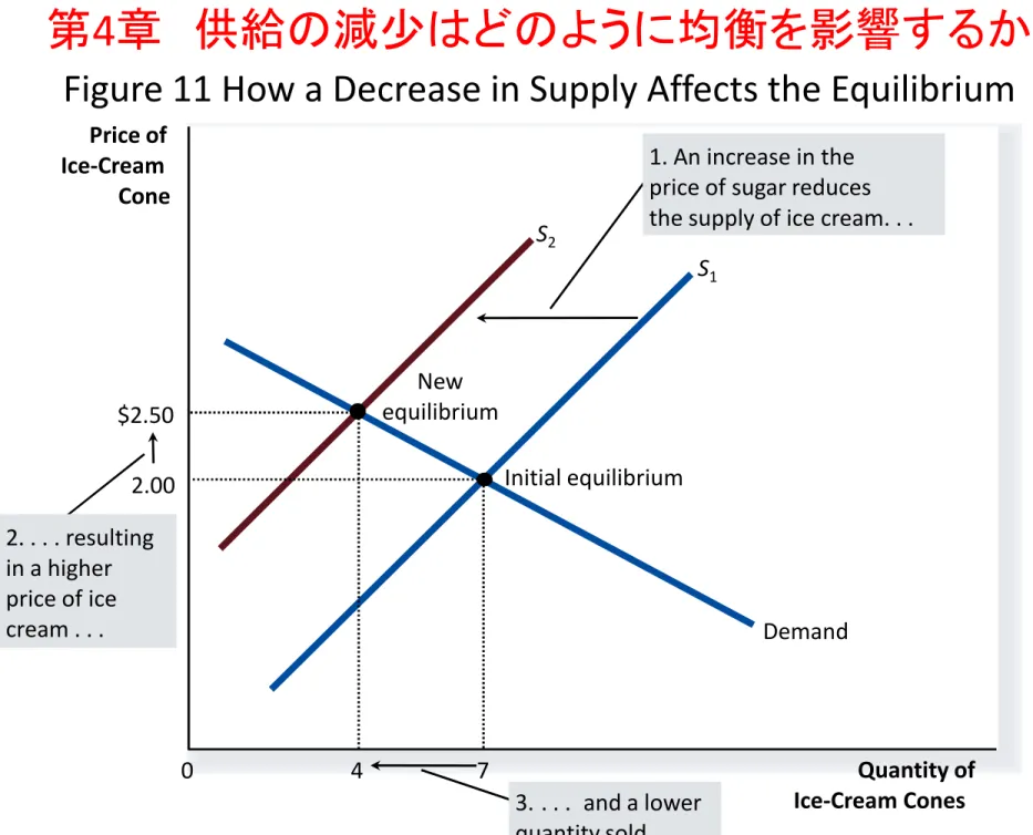
第
4章 供給の減少はどのように均衡を影響するか
Figure 11 How a Decrease in Supply Affects the Equilibrium
Price of Ice-Cream Cone 0 Quantity of Ice-Cream Cones Demand New equilibrium Initial equilibrium S1 S2 2. . . . resulting in a higher price of ice cream . . . 1. An increase in the price of sugar reduces the supply of ice cream. . .
3. . . . and a lower quantity sold. 2.00 7 $2.50 4
第
4章 クモの巣理論
第
5章 弾力性
供給の弾力性:
価格の変化に供給量の変化率を量る
尺度である。百分率で表示する。
供給の価格弾力性は供給量変化の百分率割る価格
変化の百分率。
供給量変化率(%)
供給の価格弾力性= -----------
価格変化率(%)
要注意:
需要の価格弾力性との違い:
変化は逆であり符号はプラスである。
第
5章 弾力性
供給の弾力性計算問題:ある車の価格は
100万円の場合はメー
カの生産量は
100万台である。今この商品の需要は増加した
ので価格は
110万円に上昇した。市場調査によれば、この車の
価格弾力性は2であることがわかる。それに基づいて価格の上
昇により車の
販売総量を予測ください
。
計算:
• 価格の変化率=[(
110万-100万)÷100万]×100=10%
• 販売量の変化率=(
X-100万台)÷100万台
• この車の供給の価格弾力性=
2
車供給量の増加率=
2×10%=20%
車供給量の増加分=(
20%×100万台)=20万台
車の総販売量
X
=元の
100万台+20万台=120万台
S
1D
1$10.00
500
第6章:買い手に課税
A Tax on Buyers
P
Q
D
2$11.00
P
B=
$9.50
P
S=
Tax
Effects of a $1.50 per
unit tax on buyers
新しい均衡:
税金の仕組み
税金1.5ドルを課
税すると、
Q = 450
売り手の価格
P
S= $9.50
改訂の価格
P
B= $11.00
価格の差=$1.50
= 税金
450
14
S
1第6章:売り手に課税
A Tax on Sellers
P
Q
D
1$10.00
500
S
2Effects of a $1.50 per
unit tax on sellers
アルミ生産者に$1.50課税す
ると、 per pizza.
Sellers will supply
500 pizzas
only if
P rises to $11.50,
to compensate for
this cost increase.
$11.50
Hence, a tax on sellers shifts the
S curve up by the amount of the tax.
Hence, a tax on sellers shifts the
S curve up by the amount of the tax.
15
S
1第6章:売り手に課税
A Tax on Sellers
P
Q
D
1$10.00
500
S
2450
$11.00
P
B=
$9.50
P
S=
Tax
Effects of a $1.50 per
unit tax on sellers
アルミ生産者に1
単位あたりの売り
上げに1.5ドルを
課税すると、買い
手は $11.00で買
うが、売り手は
$9.50しかもらえな
いのでアルミの生
産量は450単位ま
で減産する。
価格の差=税金
= $1.50
需要曲線Demand (private value) 私的費用Supply (private costs) 0
P
EquilibriumQ
market Quantity of Aluminium Price of Aluminium 社会的費用 Social costsQ
optimum 汚染のコスト Cost of pollutionP
Optimum第6章:練習問題 ピグー税
第
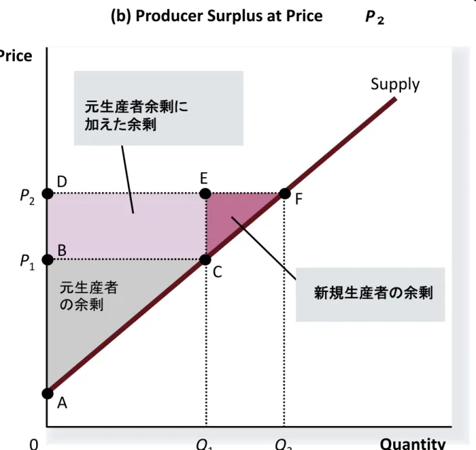
7章 生産者余剰
Figure 6 How the Price Affects Producer Surplus
Quantity
(b) Producer Surplus at Price
P
Price
0
P
1B
C
Supply
A
元生産者 の余剰Q
1P
2Q
2 新規生産者の余剰 元生産者余剰に 加えた余剰D
E
F
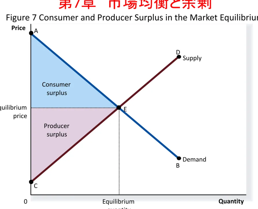
第
7章 市場均衡と余剰
Figure 7 Consumer and Producer Surplus in the Market Equilibrium
Producer surplus Consumer surplus Price 0 Quantity Equilibrium price Equilibrium quantity Supply Demand A C B D E
第
7章 市場の効率:
売り手と買い手の利益の駆動で経済を動き
Quantity Price 0 Supply Demand Cost to sellers Cost to sellers Value to buyers Value to buyersValue to buyers is greater than cost to sellers.
Value to buyers is less than cost to sellers. Equilibrium