近畿大学学術情報リポジトリ

全文

(1)（第7号）. 近畿大学理工学部研究報告. 昭和46年6月28日受理. 414によるロット不良率の推定について岩. 綺. 日出男＊. An Estimate of Lot Percent Defective by MIL-STD-414. Hideo IwASAKr* Procedures using attributes data with point estimates and confidence intervals for the percent. defective are well known.. A quality theme is to assess the performance of a production process. with respect to specifications for each product characteristic.. Therefor, estimating the percent defective and placing confidence limits on the percent defec. tive for each product characteristic has a significant meaning.. This report give a percent de. fective estimate may be determined be data with one-or two-sided assigned specification limits. 1.. Introduction. The percent defective for a quality characteristic of a given lot of product is the number of. units of product defective for that characteristic divided by the total number of units of product and multiplied by one hundred.. The quality characteristic for variables inspection is that char. acteristic of a unit of product that is actually measured, to determine conformance with a given. reguirement.. The specification limit is the requirement that a quality characteristic should meet.. This. reguirement may be expressed as an upper specification limit or a lower specification limit; or both upper and lower specification limits.. A quality theme is to assess the performance of a. production process with respect to specifications for each product characteristic.. In this sence, a quality may be defined as the probability that will fall within qiven specifica. tion limits.. The percent defective can therefor be measured by estimating the probability re—. ferred to in the definition.. The estimated lot percent defectives were obtained simply by form 2 of MIL-STD-414.. The. estimated lot percent defective shall be determined from Table B—5 for the plans based on the standerd deviation method, Table Cー5 for the plans based on the range method.. From Fig. I,. probability of acceptance in maximum allowable percent defective should be noted approach 50 percent with increase in A Q L value, and decrease in sample size is influenced considerably.. Probability of acceptance in M value with increase in sample size is stable of the order 50. percent.. The point here is dispersion or as it is commonly referred to : variation.. It is desirable,. therefor, to employ a method for estimating percent defective that will take into account such ＊. 経営工学科. -141-.

(2) variation.. Fortunately such techniques do exist, having been developed essentially for handling vanous. aspects of variables acceptance sampling. tribution of the variable.. In order to make an assumption regarding the dis. Let the quality of a product characteristic be measured as a continu. ous variable X and the process generating the characteristic be a normal population with mean µand variance a 2 .. The relation between Q and estimate the lot percent defective when enough large sample. sized is defined implicitly by. =. P = (Zrr) 21 EXP(-X 2/ 2)dx Q _ _l_. But this method for obtaining estimate is an approximate one.. not hold if the sample size is extremely small.. (1). A number of assumptions do. However, experience indicates that the tech-. Exact confidence intervals have been developed as a result of investigations of the non-central t distribution, but usually requires tedious calu. nique can be satisfactorily employed for n> 5. lations.. →. 2.. An estimate of percent defective. Then estimates of the percent defective are as follow P = Pr{x<L) +Pr(x> U}. ＝しf(x)dx + J:f(x)d L. f(x) =. （か. ",;;. 1 X=百＋ Q. p. d. f of X is. g(x) =. 入. l)r(f). 1 -(. ふり『}·〔. 。.1m 2. re り+1). 〔r(</J+2))2 .xcか3)1 （ 1-X)'.�-3J1. 『゜. m-3. 2. </J. 2. l. 芦Pr{X� � ふ{t+I}+ 1. 令） vHl〕 2. Q1vHl �Z</J g(x)dx + 1. 2. 吋X含;_9_1J_f/+ 1. ＼゜. Quv戸. :z--Z</J. QLV戸l. If guality index Q is greater than ip/ p = l). 1 ― QuvH l. 2. vm. }. g(x)dx. ＝賣誓了. [r�($訊(l-X)C$-3'./2心+� 0. l. 0. J. �=��1-X)C$-Mdx. This estimates are minimum variance unbiased estimates.. (2). For 100 (1- a) percent confidence limits on a percent defetcive characterized by two specifi. cation limits, the following two equations are solved for Pt and P2 P,.(X:;;;:Q,/引Kp州面＝（ど/2 Pr( X�Qvn[Kpハ伍） =1ーff/2. -142-.

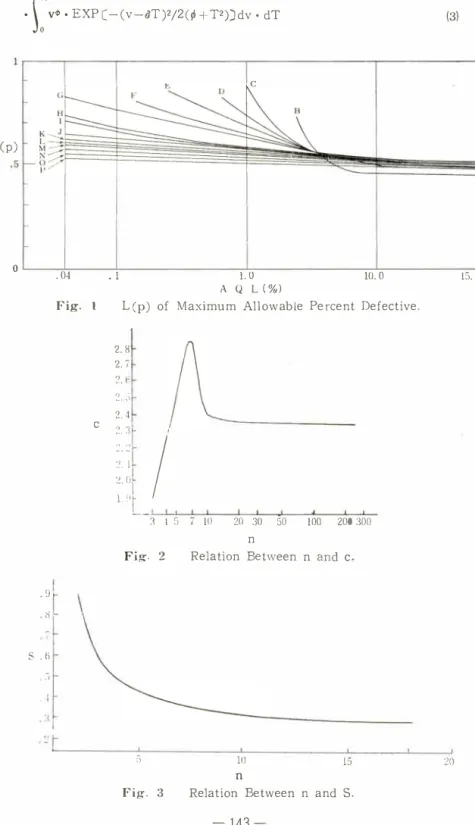
(3) Kp is defined implicitly by. =「Kp .;z;- EX P 〔匁〕 dx.. P. 1. The cumulative non-central t-distribution is Pr (T:;::::;t \iJ). 2co-l)/2V,P 1. =. t. 汀り）) (�) -. (�+ 1)/2. =. EXP(—¢炉/2 (,p +Tり〕. .) 砂• EXP C-(v-aT)2/2(,p + T2)〕 dv·dT. ゜. (3). C. L(p). 。 . 04. l. 0 A Q L (%). Fig. 1. •l. 10. 0. 15. 0. L(p) of Maximum Allowable Percent Defective.. II. 1. 3. 2. o. 5. 0 、 4 ・、. 2i. 10. 5. □. ゜゜゜ー゜. q·. c. d n a. n. n e e ＞ t e. ＼. i. e R. t a —. 2. g . l. F. nB 。゜ n. i L � 0i りi りi り. 3 7l l o. -． —. ‘ 7. 一ーーし c. ＇ー、 87 6 • • • 、 •? ) 2 2. .. 2. 4. 9 8. s . (; 、). ） . ‘. Fig. 3. Ill n. 15. Relation Between n and S.. -143-. 20.

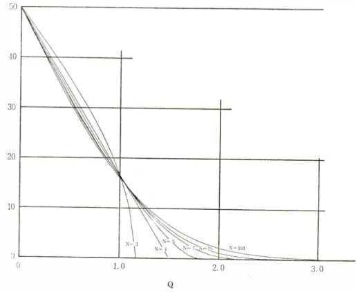
(4) so. 40. 30 〈. p紛 \ , 、 20. 10. 1.0. Fig. 4. 2.0. 3.0. Estimate of Lot Percant Defective (Standerd Deviation Method).. 50. 40. 〈. j ヽヽ P% 1 , ,. 30. 20. 10. 9l. Fig. 5. _ · �. 1. 0. Estimate of Lot Percent Defective (Range Method).. -144-. 3.0.

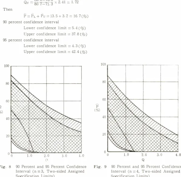
(5) Results of relation Q and P are given in Fig. 4.. As is evident (2), the percent defective is. giving a series of straight line for n = 4, a sample sige of 3 corresponds inverse proportion carve.. The maximum allowable percent defective may be approximated by normal distribution at. above n = 5.. Similarly, the relation between Q and P are given in Fig. 5 in case range method.. Estimates of the percent defective are taken to being analogous to the case of Fig. 4, and. estimates are greater in Fig. 5 case than in Fig. 4 where the sample size is not less than 7.. Therefor, percent defective can be estimated by determining plobability that quality index will. fall within required specification limits.. For range method, Fig. 2 is the relation between. factor c and sample size, and we obtain maximize c by n = 7.. The variables sampling inspec. tion plans to control the percent defective characterized have been published, for this scheme, let us investigate the relationship between S value and sample size (Fig. 3). There is an identical numerical relationship between S and l/d2 . Value d�is determined by d2 = _Jl- (1. 「. ーに(2た）. ー. 1;2 EXP(-t2/2Jdt} n_. {し(2穴）. 一. 口EXP(-t2/2Jdt} nJdx. (4). Fig. 6 give the estimates of percent defective vary as t increases for this inspection scheme,. this curve state has close tie with the normal distribution.. The graph for Q with t ((X-L)/. R·S) are shown in Fig. 7, and these lines has an incline of c/d2 what is evident on comparing. the two values.. Note that the proportion P is pre-selected and we solve for L, the lower confidence limit.. However, the type of problems we have been concerned with require an inverse arqument,. namely, a specification Limit L is assigned and at a selected confidence level a, we seek P, the minimum proportion of the population greater than L.. n3457. 50. 5. 40 4 10. 30. Q. P. 20. 20. （％） 2. 5. 4. 2. ゜. 10. t. (······normal distribution) Fig. 6 Relation Between t and P.. 3.. Confidence. Fig. 7. t. 3. Relation Between t and Q.. limit. Fig. 8, 9, 10, 11, and 12 provides a point estimate of percent defective and 90 percent confi. dence limit and 95 perceut confidence limit on the percent defective characterized by two speci. fication limits for the following sample sizes: 3, 4, 5, 10, and 100.. -145-.

(6) If an exact one-sided confidence limit alone will suffice, and this is most often the case, the. more common tables of factors for one-sided probability for normally distributed variables can. be used.. Sources for such tables which have been derived through the use of the non-central. t-distribution include references 1).. ．. Example. An characteristics are normally distributed. Lower specification L. Upper specification U. = 72. 0 = 83. 0. A random sample of 10 compoments results in sample readings having mean X = 76. 3, Xi1Ax. = 80. 7, and XMrn = 71. 3.. A point estimate of the percent defective, 90 and 95 percent confidence. interval on the percent defective are obtained as follows Q1,. Then. = 76.3—72.0 80.7-71.3. 83. 0-76. 3. Qu = 80.7-71. 3 P. "". X 2. 41. = 1. 10. X 2. 41ニ1. 72. = PL + Pu = 13. 5 + 3. 2 = 16. 7 (%) ,,. 90 percent confidence interval. Lower confidence I imit. Upper confidence limit. 95 percent confidence interval. Lower confidence limit. Upper confidence limit. ＾p. (%). = 5.4 (彩） = 37. 8 (%). = 4. 3 (彩） = 42.4 ('!6). 100. JOO. 80. 80. 60. ＾p. (%). 60 40. 20. 20. 3. 0. 4. 0. 90 Percent and 95 Percent Confidence Interval (n 3, Two-sided Assigned Specification Limits). =. 2Q. Fig. 8. ゜. 2. 0. ゜. 40. 1. 0. -―l. I. 0 Fig. 9. -146-. 3. 0. 4. 0. 90 Percent and 95 Percent Confidence Interval (n 4, Two-sided Assigned Specification Limits). =.

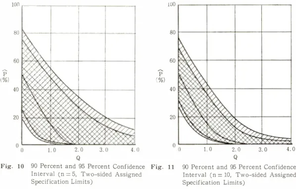
(7) 100. 100. 80. 80. 60. 60. 、`'l P% 、 _ 、. 〈. 〈. 、'， P% ’� 40. 40. 20. 20. Q 2•. 3.0. ゜. 2• Q. ゜. Fig. 10. 1. 0. 1. 0. 4.0. 90 Percent and 95 Percent Confidence Fig. 11 Interval (n 5, Two-sided Assigned Specification Limits). 3.0. 4.0. 90 Percent and 95 Percent Confidence Interval (n 10, Two-sided Assigned Specification Limits). =. =. llJO. 80. 〈. P% （. 60. ヽ�. 40. 20. 2•Q. Fig. 12. ゜. 1. 0. 3.0. 4.0. 90 Percent and 95 Percent Confidence Interval. (n 100. Two-sided Assigned Specification Limits). =. The precise method which is considered can be used for estimating percent defective and ca It is applied incases of small samples, leaving the impression that. lculating confidence limits.. acceptable results may be obtained in such cases. The method is quite cumbersame in that a table of the non-central t-distribution and a table of the Incomplete Beta Function are necessary for calculations.. -147-.

(8) 4.. Conclusion. It is desired to determine two-sided 90 and 95 percent confidence limits for the percent de. fective.. To find the lower limit PL, the PL is entered with QL by (2).. The point estimate lot. percent defective is not necessarily valid between upper and lower confidence limit, namely,. note in particular the inversion of the point estimate value and lower confidence limit value in Fig. 8, 9, and 10.. For example,. n = 3, 90 perceut confidence limit when Q = 1. 1. point estimate value is 0. 8 perceret, lower confidence limit value is 1. 1 percent.. The conventional caluculation tends to obscure the possible adverse trend which appears to. be forming ofter Q = 1. 1 (n = 3, 90 percent confidence limit) in the normal distribution approxi. mation.. Similarly, 90 percent confidence limit; n = 4,. QL> l.5. n = 3,. QL> l. 2. n = 5,. QL> L8. in case of 95 percent confidence limit; n = 4, 11 = 5,. QL>L5. QL> l.8 The method reguire that the data (samples) be randomly selected from normally distributed. populations.. 1). 2). 3). 4). 5). 6). 7). 8). References. Thomas M. Drnas, Methods of Estimating Reliability, I.Q. C, 23, 3, llS-122 (1966). R. L. Kirkpatrick, Confidence Limits on a Precent Defective Characterizedby two Specificaー tion Limits, Journal of Quality Technology, 2, 3, 150-155 (1970) United States Government Printing Office, Military Standard Sampling Procedures And Tables For Inspection By Variables For Percent Defective, (1957) Lieberman, G. J., Tables for One-sided Statistical Tolerance Limits, I. Q. C. , 14, 10, 7-9 (1958). Ellison, B . E., On Two-sided Tolerance Intervals For a Normal Distribution, A. M. S. , 35, 7記772 (1964). Owen, D. B. , A Special Case of a Bivariate Non-central t-Distribution, Biometrika, 52, 437-446 (1965). Harry R. Larson, A Nomograph of the Cumulative Binomial Distribution, I. Q. C. , 23, 6, 270-277 (1966). Irving B. Altman, The New MIL-STD-414 Sampling Inspection by Variables, I. Q. C. 14, 4, 23-26 (1957).. -148 -.

(9)