する数値シミュレーション
著者
細谷 和範, 西 隆一郎
雑誌名
鹿児島大学水産学部紀要=Memoirs of Faculty of
Fisheries Kagoshima University
巻
56
ページ
11-29
別言語のタイトル
Numerical Simulation of Tidal Currents in
Kagoshima Bay before and after the Great
Eruption in Taisho Era
ോఱڠକॲڠ໐ȁକॲȆ٬ဢڠ (Marine Biology and Oceanography Division, Faculty of Fisheries, Kagoshima University, 5-61-31 Shimo arata, Kagoshima city 9:1-1167, Japan)
* Corresponding author, Email: hosotan83@fi sh.kagoshima-u.ac.jp
ോს̤̫ͥͅఱୃఱغոஜ࡛͂ह͈
ಲၠͅ۾̳ͥତΏηντȜΏοϋ
ȁോსུ͉́͜ခତ͈غ५౷ఝ̜́ͥ߇ਗධ܅ͅ պ౾̱Ȅ̷͈౷ࠁ͉ධཤ 81kmȄୌ 36km ͈ङ͈ ޑ̞ඤს̜́ͥȅ٬ೲ౷ࠁ͉ Fig.2 ͅা̳̠͢ͅȄ211m ͈କ૬ͬ̾ს࢛͈ΏσȪն໐ȫȄड૬໐̦ 348m ͅݞ ͐ს؇໐Ȅକ૬͉ 251m ̜̦́ͥड૬໐͉ 311m ո ષͬခ̳ͥს؈́ࢹ଼̯̞ͦ̀ͥȅ̯ͣͅს؇͂ს؈ ͈͂ۼ͉ͅ໙̦ 4kmȄକ૬̦ 41m ͈॓ോକൽȪୌ ॓ോକൽȫ̦̜ͤȄુܳͅ໖ͅີ̺ͭ౷ࠁͬခ̱̞̀ ͥ2ȫȅ࡛ह͉́Ȅ॓ോକൽ̺̫̦ს؇͂ს؈֚ͬࠫ͐ ͈କႹ̞̦͂̈́̽̀ͥȄఱୃ 4 ාȪ2:25 ාȫ͈ఱୃఱ غոஜ͉Ȅ॓ോ͈௰ͅ໙̦ 511mȄ૬̯̦ 83m ͈ଳ٬ސȪ॓ോଳȫ̦̜ͤȄݱआ - ٬ګۼ͈٬କ ̦̜̹۟̽ȅఱୃఱغ͉́Ȅဣ܊̽̀͢ͅଳ٬ސ̦ ོण̯ͦͥ͂͂͜ͅȄ॓ോୌ௰͈॓ോକൽ͜ 2km ོण̱̹3ȫ ȪPlate2ȫ. ȁോს͈ಲၠ͉Ȅ٬ષ༗հͥ͢ͅ௶4ȫ,5ȫ͞ତ ΏηντȜΏοϋͥ͢ͅܡ؉͈༭࣬6ȫ,7ȫ ̥ͣȄსఘ́ ධཤ༷͈࢜؉໘ၠ̦సק̱ȄକႹ໙̦ޛ̞॓ോକൽ́ၠ ௸̦ఱ̧̞̭̦̞͂ͣͦ̀ͥȅ̹͘Ȅৗ֊൲ͅఱ̧ ̩ܙဓ̳ͥಲৄॼओၠ͉ , ს؇́শ͈۪ࠗٝͤࠁఠ ͬခ̳ͥḙ͈̏߹͉࢜٬ೲ͈౷ৗఙୟેޙ̥ͣსඤ͈ಿ ܢഎ̈́ၠ͈ͦ߹࢜ͬଔ௶̱̹ఱ࿐ͣ8ȫ͈༭֚࣬͂͜౿̱ AbstractKagoshima Bay, which is located at the southernmost part of Kyushu Island, Japan, is composed of innermost and central basins. These two basins are separated by Sakura-jima Island, which is an active volcano that had erupted heavily in 1914 in the Taisho era (so called the Taisho eruption). Before this eruption, the innermost and central basins were connected with two channels, which are named Sakura-jima Channel and Seto Strait. This eruption, however, fi lled in the Seto Strait with a large amount of lava fl ows, and mainly formed the present geometry only with Sakura-jima Channel. During 100 years after the Taisho eruption, coastal developments due to economic activities have also changed the coastal and bottom topography.
This study aims to reveal the tidal currents for the two geometries in the Meiji era before the Taisho eruption and the present period, using a numerical model based on simple assumptions. Both the simulated current fi elds showed the similar oscillating pattern. The tidal current before the Taisho eruption indicates that the phase of the oscillating fl ow in Seto Strait precedes that in Sakura-jima-Channel. This means that Seto Strait may be responsible for the balance of the current velocity intensities in the two channels. Moreover, it also infl uences the residual current pattern which is characterized by an anticlockwise rotation in the central basin.
ळგํȄ*ȁୌၦ֚
Numerical Simulation of Tidal Currents in Kagoshima Bay before and after the
Great Eruption in Taisho Era
Kazunori Hosotani* and Ryuichiro Nishi
Key words: Kagoshima Bay, Tidal current, Numerical simulation, Coastal and bottom topography, Sakura-jima
̞̀ͥȅ ȁ߃ාȄ״܅֖͈́ࠐफڰ൲͈อో൝ฺ̠ͅსඤ͈କৗ ՛ا̦࠼ැ̯̞ͦ̀ͥ9ȫȅ̫͂ͤͩს؈͉॓ോ̽̀͢ͅ ڞ̹̞̹ͦ̀ͥ͛ͅ٬କ̦తၣ̱̳̩͞Ȅକৗ՛ا̦͢ ͤࡐಠ̜́ͥḙ̷̏́Ȅକৗ٨ॐ̱͂̀Ȅ̥̾̀ంह ̱̞̹̀॓ോ௰͈ଳ٬ސ͈໘ڰͥ͢ͅს؇͂ს؈͂ ͈٬କ͈۟௯ૺا̦ুহఘͬಎͅ൦̯̹ͦḙ͈̏ ْࠗմ̞̾̀ͅఆષͣ:ȫ21ȫ ͉ს͈ੀ࿅߿ͬဥ̞̀Ȅݱ आ - ٬ګۼͅ໙ 61m ͈କႹͬٳॉ̱̹ાࣣ͈٬କ۟ ၾ͓ͬȄࡑ͈ࠫض̥ͣȄ̹̺ౙͅକႹͬٳॉ̳̺ͥ ̫͉́٬କ͉۟ୟޭഎ࣐̞ͩͦ̈́͂ͅ༭̱̞࣬̀ͥȅ ̱̥̱̦̈́ͣȄ࿅߿ࡑ͉ఱୃఱغոஜ͈ോს ͬͅठ࡛̱̹͈͉̩́̈́͜Ȅဣ܊͈ၠ̽̀͢ͅࠁ ଼̯̹࡛ͦह͈౷ࠁͅޛ̞କႹͬٳॉ̱̹ાࣣͬே̱ ̹͈̜́ͥ͜ȅح̢̀࿅߿ࡑ͉ςςႁ͈࢘ضͬࣉ ၪ̱̞̞̹̀̈́͛Ȅს؈͂ს؇͈ৗ֊൲ͅఱ̧̩גޣ ͬݞ͖̳ಲৄॼओၠ̦ບث̯̞̞ͦ̀̈́ȅ̷͈̹͛Ȅს ؈͂ს؇͈٬କ۟ͅచ̳ͥଳ٬ސ͈גޣ͉ͅ ̥̞̞̽̀̈́ḙ̷̏́Ȅུࡄݪ͉́ςςႁͬࣉၪ̱ ̹ಲၠΏηντȜΏοϋκΟσͬဥ̞̀Ȅఱୃఱغஜ ͈ྶহܢ࡛͂ह͈౷ࠁͥ͢ͅၠ͈֑̞̞ͦ̾̀ͅȄඅͅ ଳ٬ސ͈ၠ̦ͦსඤ͈ၠͦͅဓ̢ͥגޣͬྶ̥̳ͣͅ ͥȅ ȁ 2ȁ౷ࠁΟȜΗ͈ै଼͂ಲၠ͈ࠗॳ༹༷ 2/2ȁ٬ܱशକ૬͈ΟΐΗσا ȁུࡄݪ͉́Ȅତࠗॳͅဥ̞ͥକ૬ΟȜΗͬै଼̳ ً̹ͥ͛ͅݲ͈٬ͬ၌ဥ̱̹ȅঀဥ̱̹٬͉ଳ ٬ސོ̦ण̯ͦͥոஜ͈ྶহ 54 ාȪ29:: ාȫͅۏ࣐̯ ̹ͦ 21 ྔ͈ 2 ͈࣎٬ဥ٬͂Ȅ࡛ह͈౷ࠁͬయນ̯ ̵͈̱ͥ͂̀͜Ȅგ 54 ාȪ2:79 ාȫۏ࣐͈٬ͅ ଼ 25 ාȪ3111 ාȫশ͈٬܅Ȫ৽ͅࢽსߊ֖ȫܱͬ ̱̹٬ͬဥ̞̹ȅFig.3 ͅྶহܢͅݰ໐જ٬߳໐କ Ⴙޫ̽̀͢ͅै଼̯̹ͦ٬ͬা̳ȅ൚শ͈௶ၾ͉ ܻ͂२തၰڙ༹ͥ͢ͅպ౾̱࣐̞ͬȄ॑ȪυȜίȫͅ ଞ̫̹ͬ̾ଞ௶॑ͬဥ̞̀௶૬̦࣐̹ͩͦȅ̹͘Ȅ௶૬ ౙպ͉ଂȪΪυ = 2.94mȫ̜̞͉ͥ FATHOM ̜́ͥȅ ൚শِུ͉̦࣭́ڒഎ̈́٬͈ା̦ই̹̽͘ḝྶܢ́ ̜̹̦̽Ȅ࡛ह͈٬͓͂̀͜ఇ̦̞̈́௶തྟഽͬ ခ̱̞̀ͥȅ ȁ̭͈ͦͣ٬ܱशକ૬͉ະܰ௱ͅ౾̯̹ͦၗ८କ૬ ̜́ͤȄ̷͈͉́͘͘ତࠗॳͅဥ̞ͥ౷ࠁΟȜΗ̱͂ ̀၌ဥ̧̳̭̦̞̹ͥ͂́̈́͛Ȅܰ௱എ̈́Ⴅ͈ߗۼڒ ঊକ૬ͅ་̱̹۟ȅ͉̲͛ͅΟΐΗͼΎͬဥ̞̀٬ܱ शକ૬ͬΟΐΗσΟȜΗ̱͂̀උ͙ࣺ͙Ȅ̞̀උ͙ࣺ ̹ͦ͘ၗ८କ૬ͅඤொ༞ۼͬঔ̳̭͂̽̀͢ͅȄ211m
Fig.1. Bottom topography of the cross-section of Kagoshima Bay.
Fig.2. A nautical chart published in 1899. (Source: Japan Coast Guard) ۼڞ͈ߗۼڒঊକ૬ΟȜῌ་̱̹۟ȅΟΐΗͼΎ́උ ͙̹৾̽କ૬ͬ Fig.4Ȫaȫͅা̳ȅၗ८କ૬͉ાਫ਼̽͢ͅ ̀லྟ̦։̈́ͤȄ֚ഽͅ 211m ڒঊͅ་̳۟ͥ͂ાਫ਼ͅ ͉̽̀͢་۟ρȜ̦ఱၾ̱̠̭̥̀͂ͣ͘ͅȄ༞ۼ ͉ 3 ͈̾ਜ਼ͬࠐ࣐̹̀̽ȅ̴͘Ȅडౣݻၗ༹ȪNearest Neighbor༹ȫͥ͢ͅا࣐̞ͬȄၗ८౷ത͈କ૬ͬ ௶ത͈லྟͅ؊̲̀ 311m ̥ͣ 611m ྀ͈ڒঊΟȜῌ ་̱̹۟ȪFig.4Ȫbȫȫȅडౣݻၗ༹͉ΟȜΗྟഽ̦ ̞ࣞાࣣͅခ༹༷̜࢘̈́́ͥȅڎڒঊത͈କ૬͉Ȅڒঊ തͬಎͅຝ̥̹ͦౝ॑ํսඤȪࠂ R ͈ඤȫ̞ͬ ̩̥͈̾Γ·ῌߊ୨ͤȄڎΓ·Ηͬయນ̳ͥڎതȪriȫ ͈ਹ͙ັ̫̽̀͢ͅݥ͛ͣͦͥȅུࡄݪ͉́Ȅ௶ത !)b*!! ! ! ! ! !!!!!!!!! !)c*
Fig.3. Maps of bottom topography; (a) original measured data, and (b) interpolated data in 500m×500m meshes. On the left fi gure, circle (R) denotes the search region and ri denotes the distance from a grid point to each measured point.
̷̸͈ܱ͉ͦͦոئ͈փྙͬ̾ȅ ȁu,v,w : x,y,z ༷͈࢜ၠ௸ ȁH : ڎڒঊඤ͈କ૬ ȁf : ςςΩριȜΗ ȁg : ਹႁح௸ഽ ȁϼ : କպ͈་اၾ ȁP : କգ ȁЇ : ٬କྟഽȪ֚ȫ ȁNH, NV : କȪHȫ, ೄ༷࢜ȪVȫ͈־ු߸ତ ȁ̹͘Ȅೄ༷͉࢜ 4 ̱͂Ȅೄ๔͉ນ࿂̥ͣ 2,3,4 Ȫ٬ೲȫ̱̹͂ȅ༹༷͈ٜ͉ओ༹ͬঀဥ̱Ȅକ գ߃যݞ͍ f ࿂߃যͬ৾ͤව̹ͦไဥ͈ζσΙτασκ Οσ22ȫ,23ȫͬဥ̞̹ȅζσΙτασκΟσ͉Ȅచયକ֖ ͬକ૬༷̞̩̥͈࢜̾ͅͅڬ̱Ȅڎͬೄୟ̱ ̀ඤ͈ၠͬࠗॳ̳ͥκΟσ̜́ͥȅڎඤ͈ၠͦ ͉ xȄy ଼ͬ̾ඵষࡓഎ͈̱̈́͂̀͜եͩͦȄೄ༷ ͈࢜ၠ͉ͦȄڎۼ͈൲ၾͬࣉၪ̱̹ષ́Ⴒ͈̥ ͣݥͥ͘ȅ̷̱̀ၰ৪଼͈ࣣ̱͂̀ఘ̱͂̀२ষࡓഎ ̈́ၠͦા̦ນ࡛̯ͦͥȅ ȁྟഽ͈֚ၠఘͅକգ߃যͬഐဥུ̱̹κΟσ̦ນ ࡛̳ͥၠͦા͉Ȅსඤͬૺ࣐̳ͥಲৄ෨ͅచ̱Ȅڎ̦ ༷֚࢜ͅၠͦͥਜ਼գഎ̈́ၠͦા͂̈́ͥȅ̳̻̈́ͩȄ࡛ ͈࡛યͬͅ࿅̳͈͉̩݀ͥ́̈́͜Ȅს͈౷ࠁ̽͢ͅ ̀අಭັ̫ͣͦͥఱޫഎ̈́ၠ͈ͦΩΗȜϋ͈՜ͅઙത ͬࣆ̹͈̜̽́ͥ͜ȅ ȆX ༷͈࢜൲༷ ȆY ༷͈࢜൲༷ ȆZ ༷͈࢜൲༷Ȫକգ࣑ȫ ȆႲ͈ Ȇুဇນ࿂ૄ ͈லྟͅ؊̲̀٬֖̞̩̥͈ͬ̾ႀ֖̫ͅȄႀ֖ை ॑ࠂ͞ை॑ඤ͈ڬତͬഐܽ୭̱̹ȅ̷ͦ́͜౷ ࠁ་اͅచ̱̀௶തତ̦ઁ̨̳̈́ͥાࣣ͞Ȅݢੈ̈́౷ࠁ ͬ̾״܅ັ߃͉࡛́എ̞́̈́؆ඎ̦ఉ̩อ̳͈ͥ ́ȄठഽȄࡓ͈٬͂ࡉ͓̀ρȜ͂ࣉ̢ͣͦͥڒঊ କ૬ͬಈষਘୃ̱̹ȅ̞̀ȄFig.4Ȫbȫ͈ல̞ڒঊକ ૬ͅచ̱̀Ȅࠁ༞ۼ͈ΨͼςΣͺ༞ۼȪBi-linear ༞ۼȫ ͬഐဥ̱̀ 211m ۼڞ͈ڒঊͅ་̱۟Ȅ̯ͣͅȄະྶၸ ̹̈́̽ͅ٬܅͞ೄࢌ܅́ࠁ଼̯̞ͦ̀ͥࢽს൝ͬକ ૬ 1m ̱ܱ̱̹͂̀ȅ ȁ2/3ȁତࠗॳ༹༷ 2/3/2ȁΏηντȜΏοϋκΟσ ȁಲৄၠ͈ࠗॳκΟσ̱͂̀Ȅओ༹༹ٜ̳ͬ͂ͥၠ൲ κΟσͬഐဥ̱̹ȅոئͅၠͦા͈༷ܱ̳ͬȅ जດࠏ͉ܖକ࿂ͅచ̱̀ xy ࿂Ȫୌ༷࢜ͬ xȄධཤ ༷࢜ͬ y ̳͂ͥȫͬ৾ͤȄೄષ̧࢜ͅ z ͬ৾ͥȅ
2/3/3ȁޏٮૄ͂ࠗॳૄ ȁచય٬֖͈ၠͦાͬୈഽ̩͢ठ࡛̳̹͉ͥ͛ͅȄ٬֖ ͈ၠͦͬ৽̳ͥͅૄͬഐ୨ͅဓ̢̫̈́ͦ͊̈́ͣ̈́ ̞ȅඅͅȄड͜৽ါ̈́ߐ൲࡙͂̈́ͥಲৄૄ͞ૄ ͉Ȅ௶ͅܖ̧̿୭̯ͦͥຈါ̦̜ͥȅ̱̥̱̦̈́ͣȄ ًݲ͈ેޙ̦ະྶ̈́ાࣣ͉بͬဓ̢̰ͥͬං̞̈́ȅ ུࡄݪ͈ાࣣȄ൚ட̦̈́ͣȄًݲ͈ܨય͞٬યૄ͉࡛ ह͂։̜̠̱̈́ͥ́ͧȄକأ͈͞ྟഽࢹ௮̈́̓ະږ ါள̦ુͅఉ̞ḙ̷ུ̏́ΏηντȜΏοΰ͉Ȅ ݞ͍କأͥ͢ͅྟഽ་اͬࣉၪ̵̴Ȅს࢛ޏٮڒঊ ͅಲպ་൲ͬޑଷͅဓ̢ͥૄ̱̹͂ȅ ȁࠗॳͅဥ̞̹ڒঊڬͬ Fig.5 ͅȄࠗॳΩριȜΗ ͂ޏٮૄͬ Table 2 ̷̸ͦͦͅা̳ȅࠗॳڒঊ͉କ ༷̦࢜ 611m ͈ೄڒঊ̜́ͤȄს࢛໐ͅޏٮڒঊͬ୭ ̱̹ȅུ̹͘ࡄݪ͉́Ȅ৽ͅஃ̞ଳ͞କൽ͈́࿂ എ̈́ၠ͓̹ͦͬͥ͛Ȅນ࿂̥ͣ 31m ͬນ໐Ȅ31m ̥ͣ 51m ͬಎȄ̷̱̀ 51m ո૬͈ئ͈ 4 ͅڬ ̱̹ȅକ༷͈࢜־ු߸ତ͉ܡంࡃ24ȫͬ४ࣉ֚ͅ ͬဓ̢̹ȅ̤̈́ȄུκΟσ͉́Ȅೄ༷͈࢜൲ͬ ̠ඤ໐ޏٮླྀड़ႁͬକ༷࢜ၠ௸଼́ࢹ଼̯ͦͥΨ σ·́ݥ̞͛̀ͥȅޏٮૄ̞̾̀ͅȄၘ܅͈ޏٮૄ ͉Ȅڒঊ̦ல̞̭̥͂ͣΑςΛίૄ̱͂Ȅს࢛ޏٮ ૄ͉́௸ഽ࢙̦ 1 ̈́ͥͅၠૄͬ୭̱̹ȅ̹͘Ȅ ს࢛ޏٮͅဓ̢ͥಲৄૄ͉ോსඤ͈ڎಲਫ਼̤ͅ ̫ͥసקಲৄ25ȫ ̜́ͥ৽ఊ֮ਔಲȪM3ಲȫͬഐဥ ̱Ȅ87.6cm ͈૦໙་൲ͬს࢛ޏٮ́ޑଷഎͅဓ̢̹ȅ ȁ๊֚ͅȄോს͈̠̈́͢ߍࠁს͈ၠͦͬࠗॳ̳ͥषȄ ޏٮڒঊ͈୭̽̀͢ͅსࡥခ͈໗૦൲ȪΓͼΏνȫͬ ႗̳̭ܳͥ͂ͅಕփ̳ͥຈါ̦̜ͥ26ȫ ȅോს͈ΉȜ Ά͉Ȅಲৄ෨̦ٸဢ̥̲̹ͣळಿ̞სͅഥ̳࡛ͥ યͬ৾ͤե̠͈́Ȅ໗૦൲͈႗̫̹ܳͬͥ͛ͅٳޏٮ ͉ს࢛ࣣؗͅࢩ̩༷̦৾ͥၻ̞̦Ȅს࢛ٸ͈౷ࠁ͉ݢࠣ ͅ૬̩̈́ͤȄ̥̾ܳ໖̦̱̩ࠣȄഐ୨̈́ޏٮૄ͈୭ ̦ુͅඳ̱̩̈́ͥḙུ͈̹̏͛ࠗॳ͉́Ȅോსს ࢛໐́କ૬ 211m ͈Ώσ̧̦ͥධັ߃ͬޏٮڒঊ ̱͂̀୭̵̰ͥͬං̥̹̈́̽ḙ͈̏୭ͥ͢ͅ໗૦൲ ͈႗ܳેޙ͉ 4 ડ 4.2 ୯͓́ͥȅ 3ȁڒঊକ૬ͥ͢ͅྶহܢ࡛͂ह͈ോს͈٬ೲ౷ࠁ ȁུડ͉́٬̥ͣै଼̱̹ڒঊକ૬ͬဥ̞̀Ȅྶহܢ ࡛͂ह͈౷ࠁ་ا̞̾̀ͅٽၞ̳ͥȅFig.6 ࡛ͅह͈ڒ ঊକ૬̥ͣྶহܢ͈ڒঊକ૬̞̹֨କ૬ओͬা̳ȅྶহ ܢ࡛͂ह͉͂́Ȅ॓ോਔ༏͂ോঌ״܅͈౷ࠁ͈֑̞ ̦ࡐಠ̜́ͥȅၰশܢ͈କ૬ΟȜΗ͈ओȪFig.6Ȫcȫȫ͉ غ५غ̦̜̹̽॓ോͬੰ̩სఘ́ 26m ոඤ̜́ͤȄ ୈഽ͈ၻ̞௶ၾ̦̯̞̭̦̥̈́ͦ̀ͥ͂ͩͥȅ̹̺̱Ȅ ႕ٸഎͅს؈໐͈௰״܅໐́ࡉͣͦͥ 71m ոષ͈ओ ͅ۾̱͉̀Ḙ͈̏ັ߃́ఱ̧̈́౷ࠁ་ا̦ष̲̀ͅ ̞̞̭̥̈́͂ͣȄ̥͈̈́ͭͣࢋओ̜́ͥ͂ࣉ̢ͣͦͥȅ ̭͈ັ߃֚ఝ͉״܅̴̥̥ͣͩତຐ m ࣣؗ́କ૬̦֚ ܨͅ 211m ոષ་ا̳ͥݢੈ̈́σΟρ༏໐̜́ͥȅ
Fig.4. Horizontal grid spacing for the numerical model.
ྶহܢ͈٬࡛͂ह͈٬͉͂́Ȅ٬܅͈պ౾ͅ৹ۙ ͈֑̦̜̹ͥ͛Ȅ̴̥ͩ̈́պ౾͈֑̞̦ఱ̧̈́କ૬ओ ͬઉ̞̹خෝ̦̜ͥȅح̢̀ڒঊକ૬ͬै଼̳ͥष͈ ༞ۼͅ״܅౷ࠁͬठ̧࡛̱̞ͦ̈́خෝ̦̜̭ͥ͂͜ଔ ̯ͦͥȅ ȁFig.7 ॓ͅോਔ༏౷ࠁ͈ು១ͬা̳ȅଳ٬ސ͈ਔ ༏͉́ఱୃఱغ̽̀͢ͅଳ٬ސོ̦ण̯ͦȄ॓ോ͂ ఱߛോ̦͂ၘ̧̹̭̦̥̈́̽͂ͩͥͅȅ̹͘Ȅ ോঌ״܅ͬࡉͥ͂Ȅྶহܢ͈ോঌ״܅͉गຩۙ͞ګ ൝ͥ͢ͅஃ٬֖̦ධཤͅࢩ̦̞̹̦̽̀Ȅ࡛ह͉ࢽს͈ ାོ͞ၛ̀ͤ͢ͅ٬܅̦̱̯ؗͦȄକ၌ဥ̦خ ෝ̈́ޭஃ٬֖̦ࡘઁ̱̞̀ͥȅ॓ോਔ༏͈౷ࠁ་اͬ ၾഎͅ՜̳̹ͥ͛ȄFig.8 ॓ͅോକൽ͂ଳ٬ސ͈؍ ౯ݞ͍ਸ౯ͬা̳ȅକ૬̦ 41m ͂ஃ̞॓ോକൽ ͉́Ȅ॓ോ͈ဣ܊̦କ༷࢜ͅࢩ̦ͤȄ̥̾ୌ௰̥࢜̽ͅ ̀ 2km ̱̯̹̭ؗͦ͂͞Ȅോঌ͈ࢽსାͅ ฺ̞௰̥࢜̽̀ͅ٬܅̦ 2km ৻̱̯̹̭ؗͦ͂ ͤ͢ͅȄ॓ോକൽ͈໙̦߃̩̹̭̦̥̈́̽͂ͩͥͅȅ ॓ോକൽ͈౯࿂ୟȪၠୟȫ͉Ȅྶহܢ͉́ 245,511m3 ̜̹͈́̽ͅచ̱Ȅ࡛ह͉́ :1,511 m3 Ȫಎത́ া̱̹າ൮ͬ܄͛ͥ͂Ȅ 93,111 m3͂̈́ͥȫ̜́ͤȄ 44ɓȪ4:ɓȫࡘઁ̱̞̀ͥȅ༷֚Ȅଳ٬ސ͉́ဣ ܊͈ၠ̽̀͢ͅȄ٬ސོ̦ण̯̹̺̫̩ͦ́̈́Ȅ௶ B-Bȧ͈ତ km ̹ͩͤͅဣ܊̦ 261m ࢚ఙୟ̱Ȅକ࿂ ئ͈౷ࠁͬఱ̧̩་ا̵̯̹̭̦̥͂ͩͥȅ )b*! )c*!! )d*
Fig.5. Maps for digital topography (100m×100m meshes) based on nautical charts; (a) the Meiji era (1899), (b) the present period (2000), and (c) the difference between them.
Fig.6. The bird view maps of bottom topography around Sakura-jima; (a) the Meiji era (1899), and (b) the present period (2000). The aspect ratio (horizontal vs. vertical) is set to be 1:30.
Fig.7. Cross sections of (a) Sakura-jima Channel, and (b) Seto Strait. ȁ״܅֖͈ٳอฺ̠ͅஃ٬ႀ֖͈་اͬ Fig.9 ͅা̳ȅ ಎȄോঌ͈̥֙ͣܔව̹ͩͥͅ״܅֖͉́Ȅ૽ ࢥࢹ௮ً̽̀͢ͅݲ͈٬܅͈ఱ໐̦ໞ̞̩̯ͦ ̹̭̦̥͂ͩͥȅඅͅȄ५౷ߊ͞ܔව࣭زಇܖ ౷ັ߃͉́٬܅̦ 3.6km ̱̯̞ؗͦ̀ͥḙ͈̏ ͬࡓͅȄକ૬ 31m ոஃ͈ஃ٬ོ֖̤̫ͥͅၛ࿂ୟͬࠗ ॳ̳ͥ͂Ȅ 37km3 Ȫ3,711haȫ͂̈́ͥȅܔවັ߃͉́٬ ܅͈ນাպ౾̦৹ۙ։̹̈́ͥ͛Ȅོၛ࿂ୟً͉͞͞ఱ ͅࡉୟ̞͈͈ͣͦ̀ͥ͜͜Ȅോঌ͈ࢩํս́ஃ٬֖ ̦ࡘઁ̱̹̭̦̥͂ͩͥȅ 4ȁΏηντȜΏοϋࠫض 4/2ȁκΟσ͈ఏ൚͈બ ȁུΏηντȜΏοϋκΟσ͉ྟഽ̦͈֚ၠఘͬب ̱̞̭̥̀ͥ͂ͣȄࠗॳ̽̀͢ͅංͣͦͥၠͦા͉״܅ ౷ࠁͅגޣ̫̹ͬਜ਼գഎ̈́ಲၠા͂̈́ͥȅུ୯͉́Ȅ ഐဥ̱̹κΟσ͈ఏ൚ͬબ̳̹ͥ͛Ȅ௶ͥ͢ͅಲ ၠఔ͂ಲৄ૦໙ͥ͢ͅڛ࣐̹ͬ̽ȅ࡛ह͈౷ࠁͅచ ̱̀Ȅࠗॳ́ං̹ͣͦນ͈ಲၠఔͬ Fig.: ͅা̳ȅ ٬ષ༗հͥ͢ͅ௶ࠫض4ȫ ͂ࠗॳͬڛ̱̹ڎఔ ͈ၠ͉௶͂൳အ̜́ͤȄ౷ࠁͅࢰ௵̯̹ͦსඤ͈ ؉໘ၠ͈අಭͬၻ̩া̱̞̀ͥȅ̱̥̱̦̈́ͣȄΏην τȜΏοϋ̽̀͢ͅݥ̹͛ͣͦఔ͈ಿ̯͉ს࢛ັ߃͈ St.4 ͉́௶ࠫض͉ၻ̩֚౿̳͈͈ͥ͜Ȅ॓ോକൽȪSt.3ȫ ͉́ఱ̧̩Ȅ̹͘ს؈ȪSt.2ȫ͉̯̩́̈́ͥ̈́̓Ȅຈ ̴̱͜ၻ̞֚౿͉া̯̥̹̈́̽ȅ ȁষͅȄ໗૦൲ͥ͢ͅגޣ̞̾̀ͅબ̳ͥȅFig.21 ͅ ࡛ह͈౷ࠁͬဥ̞̀ࠗॳ̯̹ͦსඤڎ౷ത͈́ಲպ૦໙
͂ಲպͬা̳ȅڛచય͉ M3ಲ͈გତȪ۷௶ȫ 25ȫ ͂݊ͣ6ȫ ͥࠗ͢ͅॳࠫض̜́ͥȅࠗॳ̯̹ͦಲৄ ૦໙͉გତͤ͢͜ఱ̧̩Ȅს؈͉́૦໙̦ 21cm ఱ̧̩̞̈́̽̀ͥȅ̹͘ȄFEM ͬဥ̞̹͈݊ͣࠗॳ ུࠗ͜ॳࠫض͂൳အͅȄს؈̥࢜̽̀ͅ૦໙͈௩ح߹ ̦࢜ࡉͣͦͥȅგତນͥ͢ͅକ࿂̯͉ࣞს؈ ͕̩̓ࣞ̈́ͤȄს؈͂ს࢛́କպȪ࿂ȫओ̦ 7cm ̜ ̦ͥȄΏηντȜΏοϋࠫض͉́Ȅ̷͈ओ̦͕͂ͭ̓ࡉ ̞ͣͦ̈́ḙ͈֑̞̞̏ͦͣ̾̀ͅȄോსͬକ૬֚ ͈۰ౙ̈́ߍࠁს͂ب̳ͥ͂Ȅࡥခ૦൲ତ͉ 3.8 শۼ ͂ࡉୟͣͦͥ͜ȅࠁ૦໙෨ၑა́ນ̯ͦͥߍࠁს͈ಲ ৄ૦໙͈௩໙ၚͬ Green ༹͈௱ͤ͢ͅٽॳ̳ͥ͂Ȅსಿ
l=
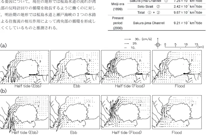
81kmȄକ૬ h =211m ུ͈ს͈ાࣣȄს؈͈ಲպ ૦໙ၚ͉ R=1/cos(kl)=1.06 ͂̈́ͥḙ̭̏́Ȅk=2π/λ ̜́ ͥȪλ ͉ಲৄ෨͈෨ಿȫȅ̳̻̈́ͩȄს࢛́ 87.6cm ͈૦ ໙ͬဓ̢̹ાࣣȄ81km ၗ̹ͦს؈͈́૦໙͉ 91.8cm ͂̈́ͥȅ٬ೲླྀड़ͥ͢ͅࠁ͈࢘ضͬࣉၪ̱̹հന ͈ͣࠫض27ȫ ̜͉̀͛̀͜ͅȄ႒য̱̹ࠫض͂̈́ͥȅ̱ ུ̹̦̽̀ΏηντȜΏοΰ͉Ȅٳޏٮ͈պ౾ͅఉ ઁ͈֑̞̦̜̽̀͜໗૦൲͈͒גޣ͉̲̞̭̈́͂ͅ ̦̈́ͥȄུࠗॳࠫض͉໗૦൲͈อͬাऐ̳ͥȄडఱ́ 21%Ȫს؈Ƚს࢛ȫ͈ಲৄ૦໙͈௩ح̦ࡉͣͦͥȅ Fig.22 ͅা̳ს࢛͈́૦໙ͬܖ̱̹͂ს͈ਸ౯ષ͈ ૦໙௩໙ၚͬࡉͥ͂Ȅ࡛ह͈౷ࠁ͉́॓ോକൽͬޏͅ૦ ໙͈ݢࠣ̈́௩حͬা̱̤̀ͤȪR=2.28ȫȄಲৄ෨͈ഥ ࠗॳً̤̞̀ͅݢੈ̈́౷ࠁષ͈କպ་൲ً̦ఱͅॳ ̯̞̭̦̥ͦ̀ͥ͂ͩͥȅ༷֚Ȅ॓ോକൽ͈໙̦ࢩ̩Ȅ ଳ٬ސ͂ඵࠏൡ͈ၠႹ̦ంह̳ͥྶহܢ͉́॓ോକൽ ັ߃͈́૦໙͈௩ح̦ဲ̢ͣͦȄR=2.25 ̞͂̈́̽̀ͥȅ ոષ͈̭̥͂ͣȄུࠗॳκΟσ͉ಲৄၠ͈අಭͬഎ ͅা̱̹͈͈͜Ȅఔ૦໙͞ს؈͈́ಲৄ૦໙͉Ȅ࡛ ͈͈͉͂͜ຈ̴̱֚͜ͅ౿̱̞̞̀̈́ȅ̱̹̦̽̀Ȅ ষ୯ոࣛͅা̳ྶহܢ࡛͂ह͈ၠ͈ͦڛ͉ȄུκΟσ͈ අષȄഎ̈́ບثͅၣ̧̤̩͓̜͛̀́ͥ͂ࣉ̢ͥȅ 4/3ȁၠͦા͈শۼ་൲ ȁFig.23 ͅྶহܢ࡛͂ह͈٬ೲ౷ࠁષ́ࠗॳ̯̹ͦນ ၠ͈ࠐশ་اͬা̳ȅၰশܢ͂͜Ȅಲպ͈་اฺ̽ͅ ̲̀ͥධཤ༷͈࢜؉໘ၠ̦సק̳ͥၠͦાͬ೮̱̀ ̞ͥȅს࢛ັ߃͞ს؇͉́Ȅ̷̸͈ͦͦၠ͈ͦΩΗȜϋ ͅఱ̧֑̞͉̈́ࡉ̞̦ͣͦ̈́Ȅ॓ോਔ༏͈ၠͦા͉͞͞ ֑̞̦ࡉͣͦͥȅ॓ോਔ༏ͬڐఱ̱̹ Fig.24 ͬࡉͥ͂Ȅ ྶহܢ̤͍࡛͢ह͈౷ࠁષ͈́ၠ͉ͦ͂॓͜ͅോକൽ ́ޑ̞ཤၠ͂ධၠ̦ࡽ̲ͥͅ؉໘ၠͬা̳̦Ȅၠ௸ ͉ྶহܢ͈༷̦ܜ̯̞ȅಲၠఔͬڛ̱̹ Fig.25 ͬࡉͥ͂Ȅ॓ോକൽ͉́ȄၠႹ̦ࢩ̞ྶহܢ͈ၠ௸૦໙ ͉࡛ह͈౷ࠁષ͈́ၠ௸૦໙ͤ͢͜ 56ɓ̯̩Ȅଳ ٬ސ͉́Ȅ 41cm/s ͈૦໙ͬခ̱̞̭̦̥̀ͥ͂ͩͥȅ ȁ̭̭́٨͛̀ Fig.24 ͅা̱̹॓ോକൽ͂ଳ٬ސ͈ ၠ͈ͦඅಭ̞̾̀ͅࣉ̢ͥȅ॓ോକൽ͈ၠ͉ͦȄၰশܢ ͂ۙ͜ಲশ͞ྖಲশ͈ഢၠশ͈́͜גޣͤ͢ͅධၠ ̹͉͘ཤၠ̦ॼၣ̱Ȅಲպ་ا͂ၠ͈ͦ་اͅպ͈ಁ ̦̲̞ͦ̀ͥȅ༷֚Ȅଳ٬ސ͈ၠ͉ͦȄಲৄ̦ഢಲ ்̳̩ͥͤ͢͜ഢၠ̱Ȅ೩ಲশࣞ͞ಲশ̤̞̀॓ͅോକ ൽ͈ၠͦ͂ݙ̧͈࢜ၠͦͬা̱̞̀ͥḙ͈̏ଳ٬ސ͈
Fig.10. M2 tide amplitude and difference of mean water level relative to Yamagawa at the mouth of the bay.
ၠ͉ͦს؇໐͂ს؈໐͈͂କպओȪFig.26ȫ̦ఱ̧̩ܙ ဓ̱̞̀ͥ͂ࣉ̢ͣͦȄ॓ോକൽ͉́Ȅྖಲশ̈́̽̀ͅ ͈͜גޣ̱̩͈̽̀͊ͣ͢ͅۼ͉କ̦ٞს؈͒͂ၠ ࣺ͚͈ͦͅచ̱ȄၠႹ̦ޛ̩؊൞͈̞͢ଳ٬ސ͉ს ؈໐͈ၠၾ͈ΨρϋΑͬ༗̠̾͢ͅܥෝ̳ͥḙ͈̏߹࢜ ͉ Fig.27 ͅা̳॓ോକൽ͞ଳ٬ސ̱̹ͬٚၠၾ͈শ
Fig.12. Simulated tidal current vectors; (a) the Meiji era (1899), and (b) present period (2000). A small fi gure embedded in the lower-left corner of each fi gure shows the phase of the tide level on the boundary at the mouth of the bay.
ࠏႥͬࡉ̥̳̞ͥ͂ͩͤ͞ȅྶহܢ͈ଳً̳ͬͥၠ ௸͞ၠၾȪს؈̥̠༷࢜࢜ͬͅୃ̳͂ͥȫ͉ಲպ̦ഢ̲ ͥஜ̥ͣݙ༷͈࢜ၠͦͬা̱̞̀ͥḙ͈̏ͦͣକႹͬ 2 ಲৄۼً̳ͥͅၠၾ͉Ȅ̷̸ͦͦȄ1.836km4 Ȫ॓ോକ ൽȫȄ1.353km4Ȫଳ٬ސȫ́Ȅၠၾ͉ 4 చ 2 ̜́ͥ ȪTable3ȫȅ̹͘Ȅྶহܢ͈କൽ͂ଳً̳ͬͥၠၾ͈ გ͉Ȅ1.:78km4̜́ͥḙ̏ͦͅచ̱Ȅ࡛ह͈౷ࠁ́ ॓ോକൽً̳ͬͥၠၾ͉ 1.:32km4 ̜́ͤȄࠗॳ́ං ̹ͣͦၰশܢ͈ს؈໐͈ၠၾ͉ఱ̧̩་̞ͩͣ̈́ȅ ȁ 4/4ȁॼओၠ ȁஜ୯͈ၠͦાͬ 2 ಲৄۼ́ا̱̹ນ͈ॼओ ၠͬ Fig.28 ͅা̳ȅ࡛ह͈౷ࠁ͉́Ȅს؇́ 7cm/s ȡ 21cm/s ͈শ͈۪̦ࠗٝͤࡉͣͦͥḙ͈̏ს؇́ শ͈۪ࠗٝͤͬা̳ॼओၠ͈ΩΗȜϋ͉Ȅ͈݊ͣࠗॳ ࠫض6ȫ7ȫ ͞ఱ࿐ͣ8ȫ ͥ͢ͅ༭֚࣬͂౿̳ͥȅ༷֚Ȅྶহ ܢ͈ॼओၠ͈ΩΗȜϋ͉শ͈۪ࠗٝͤ߹̴̦̥࢜ͩ ͙͈͈ͣͦͥ͜ͅȄ3cm/s ഽ͈৻̞ၠ̞ͦ͂̈́̽̀ͥȅ ̹͘ȄFig.29 ͅা̳॓ോ߃ཌྷ͈ڐఱͬࡉͥ͂Ȅྶহܢ ͉॓ോ͈ධ௰́শ͈ࠗٝͤॼओၠ̦͕͂ͭ̓ྫ̩Ȅଳ ٬ސਔ༏ͅ؉໘ၠ̽̀͢ͅࠁ଼̯̹ͦ͂ࡉͣͦͥܰ ࿅۪̦̈́ࡉͣͦͥȅၰ౷ࠁ͈́ს؇໐͈۪ࠁఠ̦։ ̈́ͥါ֦̞̾̀ͅȄ࡛ह͈౷ࠁ͉́॓ോକൽ͈ၠ̦ͦს ؇໐͈শ͈۪ࠗٝͤͬ੩ಿ̳̠ͥ͢ͅ൱̩͈ͅచ̱ ̀Ȅྶহܢ͈౷ࠁ͉́॓ോକൽ͂ଳ٬ސ͈ 3 ͈̾କႹ ͥ͢ͅ؉໘ၠ͈ࡽैဥ̽̀͢ͅს؇໐͈۪ͬࠁ଼̱ ̩̩̱̞͈̀ͥ͂͜ͅଔ௶̯ͦͥȅ ȁոષ͈ࠫض̥ͣȄଳ٬ސ͉॓ോକൽ͈ 2/5 ഽ͈ၠ ၾ̴̜̥̥́ͥͩͣ͜ͅȄॼओၠͅఱ̧̩ܙဓ̳ͥࠫ ضͬං̹ȅ̹̺̱ȄFig.22 ͅা̱̹̠͢ͅȄུκΟσ̦ ს؈͈ಲৄ૦໙ًͬ͞͞ఱບث̱̞̭̀ͥ͂ͬࣉၪ̳ͥ ͂Ȅඅ࡛ͅह͈॓ോକൽ͈ಲၠًͬఱບث̱̞̀ͥخෝ ̦̜ͤȄ࡛ह͈౷ࠁ́ࡉͣͦͥს؇͈۪͈ޑ̯͜৹ ًۙఱͅࡉୟ̞ͣͦ̀ͥ͜خෝ̜ͥ͜ȅ 4/5ȁρΈρϋΐͿၥঊ͈ݷ൲ ȁུ୯͉́Ȅນͅ౾̯̹ͦڒঊྀͅ 2 ࡢ͈ρΈρ ϋΐͿၥঊͬ౾̧Ȅ31 ۼ̹ͩͥͅ֊൲ેޙ͓̹ͬȅ ρΈρϋΐͿၥঊ͉Ȅນ͈ၠͦͅਲ̳ͥৗၾ̹ͬ ̞̈́بேၥঊ̱͂̀ե̹̽ȅFig.2: ͅྶহܢ࡛͂ह͈٬ ೲ౷ࠁͅచ̳ͥρΈρϋΐͿၥঊ͈ݷ൲ͬা̳ȅρΈρ ϋΐͿၥঊ͈ݷ൲͉ॼओၠͅջం̱̞͈̀ͥ͂͜ࣉ̢ͣ ͦȄၥঊ͈ΩΗȜϋ͉ Fig.28 ͈ॼओၠ͈ΩΗȜϋచ؊ ̱̞̀ͥȅ࡛ह͈౷ࠁ͉́Ȅၥঊ̦ს؇͈শ͈ࠗٝͤ ۪എ̈́ၠͦͅਲ̱̤̀ͤȄ႕̢͊Ȅܢૄ́॓ോ ͈ධ௰̜̹̽ͅၥঊ͈֚໐͉ 7 ࿒ͅܔවؗ́͘֊൲̱ ̞̀ͥȅ༷֚Ȅྶহܢ͉́Ȅს؇໐͈۪എ̈́ၠ͈ͦ ື͉ࠁ଼̯̩̩̞ͦ̈́̽̀ͥͅȅ
Fig.13. Simulated current vectors around Mt.Sakura-jima; (a) the Meiji era (1899), and (b) the present period (2000). Change in the current vector at Seto Strait indicated by a thick arrow shows a different phase referred to as Sakura-jima Channel.
Fig.14. Comparison of M2 tidal ellipses in 1899 and 2000. ȁს؈໐͉́Ȅၰ౷ࠁ͂͜ၥঊ͈ືͅఉઁ̧͈͊ͣ̾ ͉̜̦ͥȄଳ٬ސͥ͢ͅს؈͂ს؇͈͂ৗ͈֊൲͉ ڰอ͉̞́̈́ḙ͈̏ࠫض͉ఆષ:ȫ21ȫ͈ͣࡑࠫض͂ເ ࣣ̱Ȅًݲ͈౷ࠁ̦ຈ̴̱͜ڰอ̈́٬କ۟ၾͬা̳͂ ͉ࡠ̞̭ͣ̈́͂ͬাऐ̱̞̀ͥȅ̹̺̱Ȅକৗͅ߸ͥဣ ৗ͈ෛഽڐ८͉Ȅ၄ၠ̦ޑ̩̈́ͥȪτͼΦσΒ؊ႁ̦ఱ ̧̩̈́ͥȫ͕̓ڐ८߸ତ̦ఱ̧̩̈́ͤȄͤ͢ࢩ̩ڐ८̯ ͈̭͈ͦͥ́ࡠ͉̞ͤ́̈́ȅ
Fig.15. Time series of tide level and the difference of sea surface heights between St.A and St.B; (a) the Meiji era (1899), and (b) the present period (2000). St.A is located in the central basin and St.B in the innermost basin.
5ȁࣉȁख़ȁ ȁུࡄݪ͉́ྶহܢ࡛͂ह͈౷ࠁ͈ಲၠાͬڛ̱Ȅ॓ോ ଳ͈ܥෝ̽̀͢ͅȄ॓ോਔ༏͈ၠͦા̺̫̩́̈́Ȅს؇ ͈ॼओၠ͜։̈́ͥࠫضͬං̹ȅ̱̥̱̦̈́ͣȄ4.2 ୯́ ͓̹̠͢ͅȄུκΟσ͉ܳ໖ͅີ̺ͭໝॠ̈́٬ೲ౷ࠁષͬ ૺ࣐̳ͥಲৄ෨͈ഥ͈ठ࡛ͅ࿚ఴ̦̜ͤȄს؈͈ಲৄ૦ ໙ً̦͞͞ఱͅࡉୟͣͦͥ͜࿚ఴ̦̲̹ȅུડུ͉́κ Οσ͈࿚ఴത͂ࠫض͈ှ̞̾̀ͅࣉख़̳ͥȅ ȁུκΟσ͈̠͢ͅȄೄ༷͈࢜൲༷ͬഎ̈́̾ ̜̞͈ͤ́߃য̵̯ͥକգ߃যκΟσ͉ࠗॳك̦
ࠚ̞༷֚Ȅ༃࿂߃ཌྷ͈କ༷͈࢜൲գͬࣉၪ̳̭̦ͥ͂ ̧̞̹́̈́͛Ȅݢੈ̈́౷ࠁਔ༏͈କպ͞ೄၠ͈Ώην τȜΠ̦ඳ̱̞ȅඅͅၠఘ͈ྟഽུ̱̹֚ͬ͂ࡄݪ́ ͉Ȅࠗॳ̯ͦͥၠͦા͉٬࿂ષͬૺ࣐̳ͥಲৄ෨͈ਹႁ ͈͙ͅߐ൲̯ͦͥਜ਼գκȜΡ͈ၠͦ͂̈́ͤȄ͈ၠͦ ̦༷֚࢜ͅၠ͈ͦͥ́Ȅͤ͢࿚ఴ̦ࡐಠ࡛̳̞ͦ͞ͅȅ ̭͈࿚ఴ͉ඵਹङ͈ඤსͬచય̱̹ͅఈ͈٬֖͈́ ࡄݪ༭࣬́͜ࡉͣͦȪ႕̢͊Ȅຩྴ؈໐͈ম႕28ȫ ȫȄ ࿚ఴٜࠨ͈̹͈̞̩̥͈͛̾մ̦̯̞̈́ͦ̀ͥȅ႕̢ ͊Ȅ٬ೲླྀड़߸ତͬાਫ਼ͅ؊̲̀։̈́ͥͬဓ̢Ȅಲৄ ෨͈ૺ࣐௸ഽͬଷࢄ̳ͥ႕29ȫ͞Ȅ״܅ޏٮ͈ৣၚͬ ޑଷഎͅဲ̢ͥȄ̞ͩͥ͠ȦΑεϋΐႀ֖ȧͬ୭̫ͥ႕2:ȫ ̦̞̈́̓ͣͦ̀ͥȅ̱̥̱̦̈́ͣḘ༹͈༷͉̏ͦͣ ဥഎ̱̈́͂̀ͅږၛ̴̯̤ͦ̀ͣȄഐဥ̳̹ͥ ͉͛ͅఉ̩͈দ࣐॒ࢋ̦ຈါ̜́ͥȅ̱̹̦̽̀Ȅ࡛শ ത͉́ໝॠ̈́სඤ͈ၠͦͬକգ߃যκΟσٜ̩́͂ࠫ ض͈ှͅଷࡠฺ̦̰ͩͥͬං̞̈́͂এͩͦͥȅౙͅ କպ་൲͈࿚ఴٜͬࠨ̳͈̜ͥ́ͦ͊Ȅྟഽ଼ͬࣉၪ ̱̀߹գκȜΡ͈ၠͦͬࠗॳ̳̭̦ͥ͂࢘ضഎ͂ࣉ̢ͣ ̦ͦͥȄྟഽ଼̦อో̱̞̈́ൃܬ͈ΉȜΆ͉͉ͤ͞ ൳အ͈࿚ఴ̦̲̭̦ͥ͂ထே̯ͦͥḙ͈̹̏͛Ȅ ോს͈̠͢ͅޫਫ਼എͅ 4 ষࡓ̦ޑ̞ၠͦા̦ంह̳ͥ ાࣣ͉କգ߃যͬෳ̱̹ 4 ষࡓ͈κΟσͬഐဥ̱̹༷ ̦ၻ̞͂ࣉ̢ͣͦͥȅ ȁ̹̺̱Ȅକպ་൲ً̦͞͞ఱུ̹͂̈́̽κΟσ̜́̽ ̀͜Ȅಲၠ͈ιΣΒθ̞̾̀ͅഎ̈́ບث͉خෝ
Fig.16. Time series of the current velocity and the volume transport through Sakura-jima Channel and Seto Strait; (a) current velocity of the Meiji era (1899), (b) current velocity of the present period (2000), and (c) volume transport.
̜́ͥȅ႕̢͊Ȅྶহܢ͈ 3 ͈̾କႹ̦ంह̳̭ͥ͂ ́Ȅს؇͈ॼओၠ̦۪ࠁఠ̩̩̞̭ͬ͂ͤ̈́̽̀ͥͅ ͂͞Ȅଳ٬ސ͈ၠ̦ͦს؇͂ს؈͈ၠၾΨρϋΑͬ༗ ̠̾͢ͅܥෝ̳̭͉ͥ͂ၑഎͅఏ൚̜́ͥ͂ࣉ̢ͣͦ ͥȅ̹͘Ȅს؈͈କպ་൲ً̦ఱ̜࡛́ͥह͈౷ࠁ͉́Ȅ ॓ോକൽ͈ၠ௸ً̦ఱ̹͂̈́̽ࠫضȄॼओၠ̦া̳ს؇ ͈۪͈ޑً̯ͬఱͅࡉୟ̞̽̀ͥ͜خෝ̜͈ͥ͜͜ ͈ȄକႹ̦ 2 ̭۪̦̾͂̈́ͥ͂́௯̯ͦͥιΣΒθ ͈എٜ̈́৷̹͘͜ఏ൚̜́ͥ͂ࣉ̢ͣͦͥȅ ȁ 6!͂͛͘ ȁུࡄݪ͉́Ȅًݲ͈ോს͈٬̥ͣै଼̯̹ͦ ౷ࠁΟȜΗͬࡓͅȄಲৄͬٸႁ̱͂̀ဓ̢̹ତΏην τȜΏοϋ࣐̞ͬȄఱୃఱغ̦̭ܳͥոஜ࡛͂ह͈ၠ ͦાͬଔॳ̱̹ȅ৽ͅນ͈ၠͦͬບث̱̹ࠫضȄ໙̦ 4km ͈॓ോକൽͅచ̱̀Ȅ໙ 511m ͈ଳ٬ސ̦ం ह̳̭ͥ͂́Ȅ॓ോਔ༏͈ၠͦા̺̫̩́̈́Ȅს؇͈ၠ ͦ͜ͅגޣͬݞ͖̳̭̦̥̹͂ͩ̽ȅඅͅȄს؇͈শ ͈ࠗٝͤၠͦΩΗȜϋͬ̾ॼओၠ͉࡛ह͈౷ࠁ͈༷̦ ޑ̞۪ͬခ̳̭ͥ͂͞ȄρΈρϋΐͿၥঊ͈ݷ൲̦া ̱̹̠͢ͅȄს؇͂ს؈͈͂ৗ̦۟ၰশܢ͂͜ڰอ
̞̭͉́̈́͂Ȅًݲ̥࡛ͣह͈କৗ۪ޏ͈ଔ֊͓ͬͥ ષ́ਹါ̈́έ·ΗȜ̢̈́ͤͥͅȅ ȁࣽࢃȄსඤ͈କ۪ޏͬમ̱̩̹͉ͥ͛ͅȄܨય͞٬ યૄͬκΟσࣺ͙৾ͤͅȄਜ਼գκȜΡ̺̫̩́̈́Ȅ߹ գκȜΡ͈ၠͦા͜ࣉၪ̳ͥຈါ̦̜ͥȅ̯ͣͅȄໝ ॠ̈́٬ೲ౷ࠁͬૺ࣐̳ͥಲৄ෨͈ഥͬ̈́ୈഽ́Ώ ηντȜΠ̳̹ͥ͛ͅȄٸဢ֖͈גޣ̈́̓Ȅͤ͢ഐ୨̈́ ޏٮૄ͈୭͞କգ߃যͬෳ̱̹ 4 ষࡓ͈κΟσͬ ഐဥ̳ͥຈါ̦̜ͥȅ ৫ȁৃ ȁ٬͈ਓਬ̜̹ͤͅȄ٬ષ༗հ٬ဢૂ༭໐٬͈ ȆؗࢨဎঙͅͺΡΨͼΑͬೀ̞̹ఈȄോఱڠၑ ࢥڠ໐ฎআه͈ Mario P. de Leon ঙ͉ͅაै଼͈ފ ႁͬೀ̞̹ḙ̭̏ͅ૬ଃ̈́৫փͬນ̱̳͘ . ֨ဥࡃ 2ȫ ུ٬ဢڠٛȪ2:96ȫ: ུ࣭״܅٬ဢধ :882-925. 3ȫ ఱ ࢫ ຳ , ാ ઍ ֚ , ঢ় ന ࢚ , ح ࿆ , ܊ ᙎ ݅ Ȫ3115ȫ: ུਔ༏٬֖غ५။Ȫల 4 ๅȫ, ٬ဢૂ ༭໐ࡄݪ༭࣬ ,51:2-72. 4ȫ ٬ષ༗հକႹ໐Ȫ2:9:ȫ: କႹ໐۷௶༭࣬ ಲၠ۷ ௶଼ضȪგ 73 ා 5 ȡგ 74 ා 4 ȫ,356pp. 5ȫ ٬ ષ ༗ հ କ Ⴙ ໐Ȫ3114-3117ȫ: ോ ს ၠ ޙ ۷ ௶ ༭ ࣬Ȫ ഩ ঊ ๅ : http://www2.kaiho.mlit.go.jp/ KAN21/ȫ. 6ȫ କࢣྶ , ݊ࢼ࣐Ȫ3117ȫ:4 ষࡓခࡠါள༹ͅ ͥ͢ോს͈ಲၠٜଢ଼ , ോఱڠକॲڠ໐ܮ ါ ,66:2-22.
7ȫ Kikukawa,H. and N.KomakiȪ2:98ȫ:Numerical Simulation of Tide in Kagoshima Bay by Two-Dimensional Subdomain Finete Element Method, ോఱڠକॲڠ໐ܮါ ,47:288-298. 8ȫ ఱ࿐ , ்ाટ२Ȫ2:94ȫ: ോს͈ೲৗ͂౷ ࠁ - අͅೲৗ̥ͣࡉ̹ോსඤ͈٬କ͈൲̧̾ͅ ̞̀ -, ״܅٬ဢࡄݪΦȜΠ ,32Ȫ2ȫ:2-21. 9ȫ ോࡇȪ3116ȫ: ల 5 ܢോსକৗ۪ޏۯၑࠗ ْȪల 5 ܢോსήσȜْࠗȫ༭࣬ . :ȫ ఆષგ , ૩࣐ٗ , ฒ֔ୃ , ऎםহȪ2:97ȫ: ޑଷ۪ၠͥ͢ͅ٬କ۟௯ૺ͈କၑ࿅߿ࡑȽ ോს࿅߿ͥ͢ͅ൦Ƚ , ࢽსܿࡄၳ ,655:4-42. 21ȫ K.MurakamiȪ3112ȫ: ENHANCEMENT OF WATER
EXCHANGE BY ONE-WAY FLOW GENERATION,- P R O C E E D I N G S O F T H E C O N G R E S S -INTERNATIONAL ASSOCIATION FOR HYDRAULIC RESEARCH 3112,348-353. 22ȫ ಎനܔ२ , ཱ࢛ , ന࢛ࢼ֚ , ଳ࢛ణঃȪ2:94ȫ: ״܅٬֖͈२ষࡓఠȽၠఘႁڠκΟσ , ٺ࡙ ࡄݪਫ਼Ꮓ༭ ,24:22:-244. 23ȫ ಎനܔ२ , ຮ , ઐࢫຳȪ2:96ȫ: ඤს͈ၠ ൲ા͈ତࡑ , ״܅٬ဢࡄݪΦȜΠ ,24Ȫ3ȫ::7-219. 24ȫ ࣭ാજࢽსޫȪ༎ȫ Ȫ3115ȫ: ࢽსࢥম̤̫ͥͅ ృͤגޣထ௶̧͈֨ ,213pp. 25ȫ ٬ષ༗հକႹ໐Ȫ2::3ȫ:ུ״܅ಲৄგତນȄ ٬ષ༗հକႹ໐อ࣐ধ 853 :378pp 26ȫ , זനཅȄጾਕᛕȪ2:94ȫ: ಲৄࠗॳ̤̫ͅ ͥٳ༶͈ޏٮૄ̞̾̀ͅ - ౙ̈́κΟσͬ͂͜ ̱̀ͅ -, ״܅٬ဢࡄݪΦȜΠ ,32Ȫ2ȫ:66-73. 27ȫ հനਜ֚Ȫ3117ȫ: ඤს̤̫ͥͅ໗૦൲͈อ͂ခ ྶ٬͈ಲৄ௩໙̞̾̀ͅ - ໝࣣಲ͈૦ໍ̞͂ࡥခ૦ ൲͈͂ވ૦ -, ٬͈ࡄݪ ,26Ȫ5ȫ:42:-445.
Fig.18. Zoom ups of simulated residual currents on the sea surface layer; (a)the Meiji era (1899), and (b)the present period (2000).
28ȫ ခന , ࿐֚Ȫ3114ȫ: ຩྴ͈ಲৄ་൲͈ତ ΏηντȜΏοϋ , ع࢛ࡄݪ࣒ٛၳȪഩঊๅ : http://donko.civil.tohoku.ac.jp/estuary_Workshop_HP/ 3114jap.htmȫ
29ȫ Uchiyama, Y.Ȫ3115ȫ: Modeling wetting and drying scheme based on an extended logarithmic law for a three-dimensional sigma-coordinate coastal ocean modelȫ, Rep. Port and Airport Res. Inst., Vol. 54Ȫ5ȫ: 4-32. 2:ȫ I.D. JamesȪ2::2ȫ: A Primitive Equation Model
Simulation of Eddies in the Norwegian Coastal Current,Journal of Physical Oceanography,Vol.32Ȫ7ȫ :9:4-:13.