Inflection
points
and singularities
on
planar
rational cubic
curve
segments
鹿児島大学理学部酒井
宙
(Manabu SAKAI)
(Department ofMathematics, University of Kagoshima), Kagoshima, Japan 890-64*
We
obtain the distribution of inflection points and singularities on a parametricrational cubic curve segment with a great help of Mathematica (A System of for Doing
Mathematics by Computer). The reciprocal numbers of the magnitudes of the end slopes
determine the occurrence of inflection points and singularities on the segment. Its use
enables us to check whether the segment has inflection points or a singularity (a loop
or a cusp) without practical calculation the segment and to get an idea how to place
control vertices and how to choose weights for the rational B\’ezier cubic curve segment
to preserve the fair shape.
keywords: inflection points, singularities, rational cubic segments
1
Introduction
Polynomial cubic and rational cubic curves have been widely used in
computer-aided design. However, the polynomial cubic curves do not always generate “visually
pleasing”, “shape preserving” (or simply “fair”) interpolants which do not contain
un-wanted or unplaned interior inflection points and singularities to a set of planar data
points. There is a considerable literature on numerical methods for generating shape
preserving interpolations; see for example, Farin(1995), Sp\"ath$(1995\mathrm{a},1995\mathrm{b})$, and the
references therein. A way to overcome this problem is to consider the rational cubic
curve segments $z(t),$$0\leq t\leq 1,$
$u=1-t$
with a single rationality parameter $p>0$, forexample, in Sakai$(1996,1997)$
$z(t)=a_{0}t+b_{0}u+c_{0}t^{3}/(1+pu)+d_{0}u^{3}/(1+pt)$ (1.1)
and
$z(t)=a_{1}t+b_{1}u+c_{1}t^{2}u/(1+ptu)+d_{1}tu^{2}/(1+ptu)$. (1.2)
The object of this paper is to obtain the distribution of inflection points and a
sin-gularity (a loop or a cusp) on the planar rational B\’ezier cubic curve of the nonstandard
form:
$\sum_{0i=}^{3}B_{i()/}tw_{ip}i\sum_{0i=}B_{i}(t)w3i$, $B_{i}(t)=t^{i}u^{3-i}$. (1.3)
The control points $p_{i}$ belong to
$R^{2}$ and we
assume
that the weights$w_{i}$
are
all positive.We may always transform the above nonstandard form to the standard
one
with theend weights being unity by replacing $w_{i}$ with $c^{i}w_{i},$$c=\sqrt[3]{w_{0}}/w_{3}$where the new weights
correspond to the new control vertices. The present paper considers the rational B\’ezier
curve segment (1.3) in nonstandard form since (i) little difference is in the analysis by
means of Mathematica required for rational cubic segments in nonstandard and standard
forms, (ii) little difference is in complexity of representation of the obtained results, (iii)
rational B\’ezier in nonstandard form can arise, and (iv) rational segments in nonstandard
form are easier to use [Farin(1995)]. Note that it has more flexibility than the cubic
curve segments (1.1) and (1.2) since it has more degrees of freedom where the segment
(1.2) is a special case of (1.3) with $(w_{0,1}w, w_{2}, w_{3})=(1,1+p/3,1+p/3,1)$ and that
the distribution of the inflection points and singularities on (1.3) in the present paper
extends the one obtained in Sakai(1997). Sections 2-3 describe the distribution on the
rational $cubic/cubic$ curve of the form:
$z(t)= \frac{w_{0}u^{3}z_{0}+u^{2}t(w0z_{0}’+3w_{10}z)+ut^{2}(-w3Z_{1}’+3w2Z1)+w_{3}t^{3}z1}{w_{0}u^{3}+3w_{1}u^{2}t+3w2ut^{2}+w_{3}t^{3}}$ (1.4)
which satisfies Hermite data: $z^{(k)}(i)=z_{i}^{(k)},$$i=0,1,$ $k=0,1$. We derive the shape
classification of thecurvesegment (1.4) in terms of coefficients $\lambda$and
$\mu$of$\triangle z(=z_{1}-z\mathrm{o})=$
$\lambda z_{0}’+\mu z_{1}’$. In Section 4, note that the above segments (1.3) and (1.4) coincide if
$z_{0=}p_{0},$$\mathcal{Z}_{0}’=(3w_{1}/w_{0})(p_{1^{-p_{0}}}),$ $\mathcal{Z}’1=(3w_{2}/w_{3})(p_{3^{-}}p_{2}),$$\mathcal{Z}_{1}=p_{3}$. (1.5)
to obtain the distribution of inflection points and singularities (a loop and a cusp) on
the nonstandard planar rational B\’ezier cubic curve (1.3) which gives us an idea how to
place the control vertices and how to choose the weights for the fair rationalB\’ezier cubic
curve segment.
2
Inflection
points
and
singularities
on
rational cubic
curve
segments
(1.4)
In this paper, we
assume
that the tangent vectors $z_{i}’,$$i=0,1$ are not parallel,i.e., $z_{0}’\cross z_{1}’\neq 0$ where given two vectors $A=(A_{1}, A_{2}),$$B=(B_{1}, B_{2})$,
we
write $A\cross B=$$A_{1}B_{2}-A_{2}B_{1}$. Note that if $z_{i}’,$$i=1,2$
are
not parallel, then $\triangle z(=z_{1}-z_{0})$ can berepresented as $\triangle z=\lambda z_{0}’+\mu z_{1}’$ where $(\lambda, \mu)$
are
easily determined from the given data,i.e., $(\lambda, \mu)=(\triangle z\mathrm{X}z_{1}’, -\triangle z\mathrm{x}z_{0}’)/(z_{0}’\mathrm{x}z_{1}’)$. The coefficient are to be considered
to be “ reciprocal numbers of the magnitudes of the end slopes”. Use of these $\lambda$ and
$\mu$ gives simpler shape classification than traditional use of of the magnitudes of $1/\lambda$
distributionofinterior inflectionpoints and singularities
on
the parametricrational cubicsegment (1.4). In order to display the
occurrences
of inflection points and singularitiesdepending on these parameters, we introduce
an
auxiliary plane with the coordinates$\lambda$ and
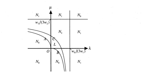
$\mu$. In Figure 1, the plane is divided into several regions by the
$\lambda$-axis, the
$\mu$-axis, the straight lines $\lambda=w_{0}/(3w_{1})$ and $\mu=w_{3}/(3w_{2}),$
$A(\mathrm{t}\mathrm{h}\mathrm{e}$ segment of the
hyperbola): $w_{0}\mu^{2}=\lambda(3w_{2}\mu-W_{3})$ limited by the second quadrant and $B(\mathrm{t}\mathrm{h}\mathrm{e}$ segment
of the hyperbola): $w_{3}\lambda^{2}=\mu(3w_{1}\lambda-w_{0})$ limited by the fourth quadrant and the
curve
$C$ is $(u(\sigma), v(\sigma)),$ $0<\sigma<\infty$:
(i) $u( \sigma)=\frac{w_{0}(-w0^{\sigma^{4}}+3w2\sigma+2w_{3}\sigma)2}{3\{2w_{0}w_{2}\sigma+(33w_{1}w_{2}+w0w3)\sigma+2w_{1}w3\sigma 2\}}$
(2.1) (ii) $v( \sigma)=\frac{w_{3}(2w0\sigma^{3}+3w_{1}\sigma-2w3)}{3\{2w0w2\sigma^{3}+(3w1w2+w0w_{3})\sigma^{2}+2w1w3\sigma\}}$ .
Mathematica helps us check that the
curve
$C:(u(\sigma), v(\sigma)),$$0<$ a $<\infty$ is a branch of$k(\lambda, \mu)=0$ limited by $\lambda<w_{0}/(3w_{1}),$$\mu<w_{3}/(3w_{2})$:
$k(\lambda, \mu)=4w_{30}^{2}w(3w_{2}\mu-w_{3})\lambda 3+4w^{2}w3(03w1\lambda-w\mathrm{o})\mu-33(w_{0}w3\lambda\mu)^{2}$ (2.2)
$+\{(3w_{1}\lambda-w_{0})(3w2\mu-w3)\}2-6w_{0}w_{3}(3w_{1}\lambda-w_{0})(3w_{2}\mu-w3)\lambda\mu$.
$k(\lambda, \mu)=0$ has two straight lines $\lambda=w_{0}/(3w_{1})$ and $\mu=w_{3}/(3w_{2})$ as its asymptotic
lines.
Theorem 1 Assume that $\triangle z=\lambda z_{0}’+\mu z_{1}’$ with $z_{0}’\cross z_{1}’\neq 0$. Then, Figure 1 gives the
distribution
of inflections
and singularity on the curveof
theform
(1.4) with respect to$(\lambda, \mu)$ where (i) $N_{i},$$0\leq i\leq 2$ represent the regions
for
which the curve hasi-inflection
points and no singularity, (ii) $C$ (or$L$ limited by$A,$$B,$$C$) means the region
for
the curveto have a cusp (ora loop) and no
inflection
point. The region$N_{0}$ contains the boundaries$A$ and $B$; and $N_{1}$ contains the two straight lines: $\lambda=w_{0}/(3w_{1}),$ $\mu<w_{3}/(3w_{2})$ and
$\lambda<w_{0}/(3w_{1}),$$\mu=w3/(3w_{2})$.
The implicit form (2.2) is
more
useful when determining on which side of thecurve
the point $(\lambda, \mu)$ lies, while the parametric form (2.1) is
more
useful for displaying thecurve.
When $(w_{0}, w_{1}, w_{2}, W3)=(1,1,1,1)$ (i.e., the polynomial cubic case), $A,$ $B$are $\mu^{2}=\lambda(3\mu-1),$$\lambda^{2}=\mu(3\lambda-1)$, and $C$ reduces to a branch of the hyperbola:
$(\lambda-1/3)(\mu-1/3)=1/36$ limited by $\lambda,$ $\mu<1/3$. In another paper, Mathematica will
determine
a
subregion $(\in N_{0)})$ in the first $\mathrm{q}\mathrm{u}\mathrm{d}\mathrm{r}\dot{\mathrm{a}}\mathrm{n}\mathrm{t}$ for the parametric cubic segment tobe a spiral of monotone curvature having several advantages of containg nether
inflec-tion points, singularities
nor
curvature extrema;see
Figure 1. Herewe
give the resultwithout its proof: the $T$-cubic spline is a spiral if and only if $(\lambda-1/2)(\mu-1/2)\leq$
$0,$ $(\lambda-1/3)(\mu-1/3)\geq 1/36$. The spiral is useful as a transition
curve
between straightline segment and circular
arc
segment, and between circulararc
segments of differentradii and is also used in data fitting.
: Theorem 1 saysthat the rational “$cubic/cubic$”
curve
has thesame
behavior (theFig. 1. Distribution of infiections and singularity.
3
Proof of Theorem 1
Inflection points: Let $\varphi(t)$ be the denominator of(1.4), i.e., $\varphi(t)=w_{0}u^{3}+3w_{1}u^{2}t+$
$3w_{2}ut^{2}+w_{3}t^{3}$. Use $\triangle z=\lambda z_{0}’+\mu z_{1}’$ to obtain
$\varphi(t)^{2_{Z’}}(t)$ $=$ $a(t)_{Z_{0}’}+b(t)z’1$ (3.1) $\varphi(t)^{3\prime/}z(t)$ $=$ $\{a’(t)\varphi(t)-2a(t)\varphi’(t)\}Z_{0}/+\{b’(t)\varphi(t)-2b(t)\varphi/(t)\}_{Z_{1}’}$ where $a(t)=u(w_{0^{u^{3}-3w}0\mathrm{s}}^{2}0w_{2}t^{2}u-2wwt)3+3\lambda tu(2w0w_{2}u2+3w_{1}w_{2}tu+w_{0^{w}3}tu+2w_{1}w_{3}t^{2})$ (3.2) $b(t)=t(w_{31}^{3}t^{3}-3ww3tu^{2}-2w_{0}w_{3}u^{3})+3\mu tu(2w0w2u2+3w_{1}w_{2}tu+w_{0^{w}3}tu+2w_{1}w_{3}t^{2})$
Inflection points on (1.4) are determined by $z’(t)\cross z’’(t)=0,0<t<1$ or $a’(t)b(t)-$
$a(t)b’(t)=0,0<t<1$
. Mathematica helps us check that substitution of $t=1/(1+$$\sigma),$$0<\sigma<\infty$ equivalentlyrewrites the above determining equation$a’(t)b(t)-a(t)b/(t)=$
$0$ of degree six as a product of two cubic polynomials:
$\{w_{0}^{2}(3w2\mu-w_{3})\sigma 3+3w_{0^{w_{3}}}^{2}\mu\sigma^{2}+3w0w^{2}\lambda\sigma 3+w_{3}^{2}(3w_{1}\lambda-w_{0})\}\varphi(\sigma)=0$. (3.3)
Since $w_{i}>0,0\leq i\leq 3$, from above
we
obtaina
cubic equation:$w_{0}^{2}(3w2\mu-w3)\sigma+3w_{0}^{2}w3\mu\sigma^{2}+3w_{03}w32\lambda\sigma+w_{3}(23w1\lambda-w_{0})=0$. (3.4)
The number of the inflection points being equal to the number of the simple positive
roots of the cubic equation (3.4), easily
we
have(b) $\{\lambda-w_{0}/(3w_{1})\}\{\mu-w_{3}/(3w_{2})\}<0$ or $\lambda=w_{0}/(3w_{1}),$$\mu<w_{3}/(3w_{2})$ or $\lambda<$ $w_{0}/(3w_{1}),$$\mu=w3/(3w_{2}):(\lambda, \mu)\in N_{1}$.
(c) $\lambda<w_{0}/(3w_{1}),$$\mu<w_{3}/(3w_{2})$: Descartes’ Rule ofSigns implies that the number of
the positive roots of (3.4) is either zero or two, counting any double root twice. Remark
that $(\lambda, \mu)$ is on the boundary between these
cases
ifa double rootoccurs.
At a positivedouble root $\sigma$, the cubic (3.4) and its first derivative must vanish, which gives two
equations that
are
linear in $\lambda$ and$\mu$:
$3w_{3}^{2}(w0^{\sigma}+w_{1})\lambda+3w_{0}^{2}(W2\sigma+W3\sigma)32=\mu W0^{w(_{W_{0}}\sigma+w_{3})}33$
(3.5) $w_{0}w_{3}^{2}\lambda+w_{0}^{2}(3w_{2}\sigma^{2}+2w_{3}\sigma)\mu=w^{2}w\sigma 032$
Thus it is straightforward to identify the required boundary: $(\lambda, \mu)=(u(\sigma), v(\sigma))$.
Tak-ing into account of the signs of the coefficients of (3.4), $(\lambda, \mu)\in N_{0}$ for $\lambda=u(\sigma),$$\mu\leq v(\sigma)$
and $(\lambda, \mu)\in N_{2}$ for $\lambda=u(\sigma),$ $\mu>v(\sigma)$, respectively. Hence we have
Lemma 2
If
$(\lambda, \mu)\in N_{i},$$0\leq i\leq 2$, the curve (1.4) has $i$-inflection
$point\mathit{8}$ where $N_{0}=${
$(\lambda,$$\mu)|\lambda\geq w_{0}/(3w_{1}),$$\mu\geq w_{3}/(3w_{2})$ or $k(\lambda,$ $\mu)\geq 0,$$\lambda\leq w_{0}/(3w_{1}),$ $\mu\leq w_{3}/(3w_{2})$},
$N_{1}=\{(\lambda, \mu)|(\lambda-w_{0}/(3w_{1}))(\mu-w3/(3w_{2}))\leq 0$ or $\lambda=w_{0}/(3w_{1}),$$\mu<w_{3}/(3w_{2})$ or $\lambda<$
$w_{0}/(3w_{1}),$$\mu=w_{3}/(3w_{2})\}$ and $N_{2}=\{(\lambda, \mu)|k(\lambda, \mu)<0, \lambda<w_{0}/(3w_{1}), \mu<w_{3}/(3w_{2})\}$.
Singularities: A loop occurs if $z(\alpha)=z(\beta)$ for $0<\alpha<\beta<1$. Since $z_{0}’$ and $z_{1}’$ are
independent, letting the coefficients of the two vectors in $\{z(\alpha)-z(\beta)\}$ be zero gives
$\lambda[\beta^{2}\{w_{3}\beta+3w2(1-\beta)\}\varphi(\alpha)-\alpha^{2}\{w3\alpha+3w2(1-\alpha)\}\varphi(\beta)]$
$=w_{0}\{(1-\alpha)2\alpha\varphi(\beta)-(1-\beta)^{2}\beta\varphi(\alpha)\}$
(3.6)
$\mu[\beta^{2}\{w_{3}\beta+3w2(1-\beta)\}\varphi(\alpha)-\alpha^{2}\{w3\alpha+3w2(1-\alpha)\}\varphi(\beta)]$
$=w_{3}\{(1-\beta)\beta 2\varphi(\alpha)-(1-\alpha)\alpha^{2}\varphi(\beta)\}$.
Note $\alpha\neq\beta$ to obtain from the above (3.6)
$\lambda/w_{0}$ $=$ $\{-w_{0}(1-\alpha)2(1-\beta)^{2}+w_{3}\alpha\beta(\alpha+\beta-2\alpha\beta)+3w_{2}\alpha\beta(1-\alpha)(1-\beta)\}/D$ (3.7) $\mu/w_{3}$ $=$ $\{w_{0}(1-\alpha)(1-\beta)(\alpha+\beta-2\alpha\beta)-w3\alpha^{2}\beta^{2}+3w_{1}\alpha\beta(1-\alpha)(1-\beta)\}/D$ with $D=w_{0}w_{3}\{\beta^{2}(1-\alpha)^{2}+\alpha\beta(1-\alpha)(1-\beta)+\alpha^{2}(1-\beta)^{2}\}+3w_{1}w_{3}\alpha\beta(\alpha+\beta-2\alpha\beta)(3.8)$ $+3w_{0^{w}2}(1-\alpha)(1-\beta)(\alpha+\beta-2\alpha\beta)+9w_{1}w_{2}(1-\alpha)(1-\beta)\alpha\beta$. where $0<\alpha<\beta<1$. (3.9)
Hence, we consider the image of $(\lambda, \mu)$ by $(3.7)-(3.8)$ under (3.9) to get the necessary
and sufficient conditions for the existence of the loop
on
(1.4). First the image of theboundary of the region determined by inequalities (3.9) is given by:
(i) $\alpha=0,0<\beta<1\Rightarrow w_{0}\mu^{2}=\lambda(3w_{2}\mu-w_{3})$
(ii) $0<\alpha<1,$$\beta=1\Rightarrow w_{3}\lambda^{2}=\mu(3w_{1}\lambda-w_{0})$ (3.10)
(iii) $0<\alpha=\beta<1$ or $\alpha=\beta=1/(1+\sigma),$$0<\sigma<\infty\Rightarrow(\lambda, \mu)=(u(\sigma), v(\sigma))$.
Next, Mathematica helps us check that the Jacobian matrix of $(\lambda, \mu)$ with respect to
$(\alpha, \beta)$ is nonsingular for $(\alpha, \beta)=(1/(1+c), 1/(1+d)),$
$0<d<c$
as follows;$\{3w_{0}w_{2}cd(c+d)+(w_{0}w_{3}+9w_{1}w_{2})Cd+3w_{1}w_{3}(c+d)+w_{0}w_{3}(c^{2}+d^{2})\}^{3}$
$=(d-C)\{W_{0}W_{3}(1+c)(1+d)\}^{2}(w_{0}c\mathrm{s}+3w_{1}c^{2}+3w_{2}c+w_{3})\cross$ (3.11) $(w_{0}d^{3}+3w_{1}d^{2}+3w_{2}d+w_{3})$ $(<0)$.
Note that a cusp on a curve can be regarded as the limit ofa loop to obtain
Lemma 3
If
$(\lambda, \mu)\in L$ or $C$, then a loop or a cusp occurs on the curve segment(1.4) where $L=\{(\lambda, \mu)|k(\lambda, \mu)>0,$ $\lambda<w_{0}/(3w_{1}),$$\mu<w_{3}/(3w_{2}),$$W3\lambda^{2}>\mu(3w_{1}\lambda-$
$w_{0}),$ $w_{0}\mu^{2}>\lambda(3w_{2}\mu-w_{3})\}$.
Lemmas 2-3 give the desired Theorem 1 on the distribution of inflection points and
singularities on the planar rational cubic curves of the form (1.4) where note that the
inflection points, cusps or loops do not occur simultaneously.
4
Shape
classification of rational cubic
B\’ezier
curve
As in (Meek
&Walton,1990),
we want to know the shape classification of therational cubic curve (1.3) in terms of one of the control vertices. Based on Theorem 1,
we
consider the distribution of inflection points and singularities on the rational cubicB\’ezier curve (1.3) or the shape of the curve segment resulting from placing$p_{1}$ in various
regions of the plane, with$p_{0},p_{2},p_{3}$ and $w_{0},$ $w_{1},$ $w_{2},$$w_{3}$
. fixed. From (1.3), we equivalently
$\mathrm{r}\mathrm{e}\mathrm{w}\mathrm{r}\mathrm{i}\mathrm{r}\mathrm{e}\triangle z=\lambda z_{0}’+\mu z_{1}’$ as
$p_{3}-p_{0}=(3w_{1}/w_{0})\lambda(p_{1^{-}}p0)+(3w_{2}/w_{3})\mu(p_{3}-p2)$ (4.1)
from which follows
$p_{1}-p_{2}=u(p\mathrm{o}^{-}p2)+v(p_{3}-p2)$, $u=1- \frac{w_{0}}{3w_{1}\lambda},$$v= \frac{w_{0}}{3w_{1}\lambda}(1-\frac{3w_{2}\mu}{w_{3}})$, (4.2)
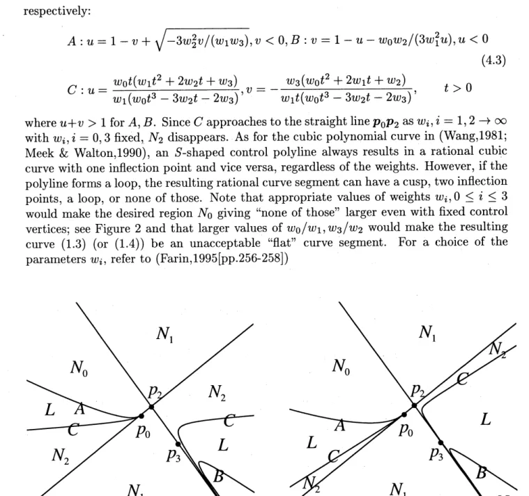
Theorem 1 gives Figure 2 (the shape classification of the rational cubic B\’ezier
curve
forrespectively:
$A:u=1-v+\sqrt{-3w_{2}^{2}v/(w_{1}w_{3})},$$v<0,$$B:v=1-u-w0w2/(3w_{1}u)2,$$u<0$
(4.3) $C$
:
$u= \frac{w_{0}t(w1t2+2w_{2}t+w3)}{w_{1}(w_{0}t\mathrm{s}-3w2t-2w_{3})},$ $v=- \frac{w_{3}(w_{01}t^{2}+2wt+w_{2})}{w_{1}t(w0^{t^{\mathrm{s}}}-3w_{2}t-2w_{3})}$, $t>0$where$u+v>1$ for$A,$$B$. Since $C$approachesto the straight line$p_{0}p_{2}$
as
$w_{i},$ $i=1,2arrow\infty$with $w_{i},$$i=0,3$ fixed, $N_{2}$ disappears. As for the cubic polynomial
curve
in (Wang,1981;Meek
&Walton,1990),
an $S$-shaped control polyline always results in a rational cubiccurve
with one inflection point and vice versa, regardless of the weights. However, if thepolylineforms aloop, the resultingrational
curve
segmentcan
havea
cusp, two inflectionpoints, a loop, or none of those. Note that appropriate values of weights $w_{i},$$0\leq i\leq 3$
would make the desired region $N_{0}$ giving “none of those” larger even with fixed control
vertices; see Figure 2 and that larger values of $w_{0}/w_{1},$ $w_{3}/w_{2}$ would make the resulting
curve (1.3) (or (1.4)) be an unacceptable ($‘ \mathrm{f}\mathrm{l}\mathrm{a}\mathrm{t}$”
curve
segment. For a choice of theparameters $w_{i}$, refer to (Farin,$1995[\mathrm{p}\mathrm{p}.256-258]$)
Fig. 2. Shape classification with $(w_{0}, w_{1,2}w, w_{3})=(1,4/3,1,1)$ and (1, 16/3, 4, 1)
In order to obtain the shape classification of the rational cubic B\’ezier
curve
forplace-ment of from placing$p_{3}$ in various regions ofthe plane, with$p_{0},$$p_{1},p_{2}$ and $w_{0},$$w_{1,2}w,$ $w_{3}$
fixed, we only have to rewrite (4.1)
as
$p_{3^{-}}p_{2}=u(p0-p_{2})+v(p_{1}-p2)$, $u= \frac{w_{3}(w_{0^{-3w}1}\lambda)}{w_{0}(w_{3^{-}}3w_{2\mu})},$$v= \frac{3w_{1}w_{3}\lambda}{w_{0}(w_{3^{-}}3w_{2\mu})}$ (4.4)
Acknowledgment
Manitoba, Canada $\mathrm{R}3\mathrm{T}2\mathrm{N}2$ for his valuable comments and suggestions.
References
Wang, C.Y. (1981), Shape classification of the parametric cubic curve and parametric
B-spline curve. Comput. Aided-Des.13,199-206.
Farin, G. (1995), Curves and Surfaces for Computer Aided Geometric Design-Practical
Guide. Academic Press, New York.
Meek, D.S.
&Walton,
D.J. (1990), Shape determination of planar uniform cubic B-splinesegments. Comput. Aided-Des. 22, 434-441.
Sakai, M.
&Usmani,
R.A. (1995), On fair parametric rational cubic curves. BIT 36,349-367.
Sakai, M (1997), Inflections and singularity on parametric rational cubic curves. Numer.
Math.76, 403-417.
Sakai, M. Inflection points and singularities on planar rational cubic curve segments. (to
appear in Computer Aided Geometric Design).
Sakai, M. Planar Hermite spiral interpolation (submitted).
Stone, M.C.
&DeRose,
T.D. (1989), Characterizing cubic B\’ezier curves. ACMTransac-tion
on Graphics 8, 147-163.
Sp\"ath, H. (1995), One Dimensional Spline Interpolation Algorithms. AK Peters
Welles-ley,
Masasachusetts.
Sp\"ath, H. (1995), Two Dimensional Spline Interpolation Algorithms. AK Peters
Welles-ley,
Masasachusetts.
B. -Q. Su.