Distributed Motion Generation for Carrying a Ladder by Two Omni-Directional Robots (Algorithm Engineering as a New Paradigm)

Distributed

Motion

Generation for

Carrying a

Ladder

by Two

Omni-Directional

Robots

Yuichi

Asahiro1

,

Eric

Chung-Hui

Chang2,

Amol

Mali2

, Syunsuke

Nagafuji1

, Ichiro $\mathrm{S}\mathrm{u}\mathrm{z}\mathrm{u}\mathrm{k}\mathrm{i}2$,

and

Masafumi

YAMASHITA1

1Dept.

ofComputerScience and Communication Engineering, Kyushu University

6-10-1 Hakozaki, Higashi-ku Fukuoka, 812-8581, Japan

{as

$\mathrm{a}\mathrm{h}\mathrm{i}$ro@, nagafuji@tcslab. ,

mak@}

$\mathrm{c}\mathrm{s}\mathrm{c}\mathrm{e}$

.

kyushu-u.$\mathrm{a}\mathrm{c}.\mathrm{j}\mathrm{p}$

2 _{Dept. of Electrical Engineering and Computer Science}

University of Wisconsin-Milwaukee, Milwaukee, WI 53201, $\mathrm{U}.\mathrm{S}$.A.

{ecchang, mali, $\mathrm{s}\mathrm{u}\mathrm{z}\mathrm{u}\mathrm{k}\mathrm{i}$

}

$@\mathrm{C}\mathrm{s}.\mathrm{u}\mathrm{w}\mathrm{m}.\mathrm{e}\mathrm{d}\mathrm{u}$

Abstract: The problem of moving a pairofomni-directional robots carrying a ladder using

distributed control is discussed. We first consider the case in which two robots that may

differ only in their maximum speeds are situated in an obstacle-free workspace, and present

two distributed algorithms. Next, a distributed algorithm is presented for the casein which

the workspace is a narrow corridor with a 90 degree corner and two robots

are.chosen

from

a large pool of robots having different characteristics in terms of the maximum speed, path

generation strategy, sensitivity to the motion of the other robot, etc. The effectiveness of the

algorithms is evaluated using computer simulation.

Keywords: distributed control, mobile robots, transportation

1

Introduction

There are two general approaches for

control-ling multiple robots transporting an object. One

is the centralized approach in which the motion

of the robots is generated by an outside entity

that can observe the global state of the system

$[7, 12]$

.

The other is the distributed approach,

where everyindividual robot hastodecide its

mo-tion based on thelocal information available to it

$[8, 9]$. This paper discusses the problem of

trans-porting a ladder, or any long object such as a

rocket and a bridge, using two omni-directional

robots under distributed control.

Within the framework of the centralized ap-proach, it is possible to compute a time-optimal motion of two such robots in an obstacle-free

workspace using optimal control theory, under

the assumption that the speed of the robots is

either $0$ or a given constant at any moment

dur-ing a motion $[5, 10]$

.

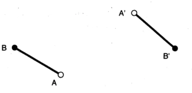
Fig. 1 shows a instance of

this problem in which robots located at $A$ and $B$

must move to$A’$ and $B’$, respectively, and a

time-optimal motion for this instance obtained by this

method is shown in Fig. 2. Unfortunately, the

applicability of this method for actually moving

physical robots in optimal time is somewhat

lim-ited, because (i) the method uses complex

calcu-lation involving elliptic integral, and (ii) physical

robots cannot always execute a computed

mo-tion precisely –they can neither accelerate to

the maximum speed instantaneously, nor move

along a given trajectory precisely dueto

mechan-ical imprecision and the unpredictability of the

environment (suchas aslight incline of the floor).

In contrast, in the distributed approach the

robots can cope with unexpected perturbation by

continuously monitoring their progress and

dy-namically adjusting their trajectories. The

over-all motion resulting from such a distributed

strat-egy can be $\mathrm{n}\mathrm{e}\dot{\mathrm{a}}$

rly as efficient as an optimal

mo-tion $[1, 2]$

.

One should also keep in mind,

how-ever, that good distributed algorithms are

usu-ally much harder to design than centralized algo-rithms. For instance, the fact that the path of

neither robot is straight in the optimal motion

of Fig. 2 indicates that efficient motion may not

be attainable distributively if either robot

sim-ply attempts to reach its destination as quickly

“adherence” to stay on the intended path, and reaction to the other robot’s motion.

Figure 1: An instance of the ladder carrying prob-lem.

Figure 2: Time-optimal motion for the instance

shownin Fig. 1.

A number ofdistributed algorithms for

carry-inga ladder using two identical omni-directional

robots (hence having the

same

maximumspeed)

have been reported for the case in which there

are noobstacles in the workspace$[1, 2]$

.

The goal

of this paper is to consider the problem under

the assumption that the robots are not

necessar-ily identical and the workspace is not necessarily

obstacle-free. Specifically:

1. We present two distributed algorithms for

thecase in which two robots possibly having

different maximum speeds are situated in an

obstacle-free workspace. The first algorithm,

ALGI, assumes that each robot knows the

maximum speeds of both robots, while the

second algorithm, ALG2, is for the case this

information is not available. The algorithms

are

evaluated using computer simulation.

2. We then present and evaluate an algorithm

calledALG3for thecasein which two robots

must transport a ladder through a corridor

with a 90 degree corner. We assume that

the two robots

can

have different

charac-teristics in terms of the selection of a path

through the corner, the maximum speed,

Due to space limitation we are not able to

present some of the details. The missing details

may be found in the references, orwill be reported

in forthcoming papers.

2

The

Model

The model of the robots we use is based on the

omni-directional robots developed at RIKEN [3].

We represent each robot $R$ as a disk. One end

of the ladder is attached to a force sensor that

we model as an ideal spring located at the center

of $R$

.

At any time during a motion the vector

from the center of $R$ to the tip of the ladder

at-tached to its force sensor is called the

_offset

vec-$tor$, and is denoted $\mathit{0}arrow$

.

The term

offset

refers to

$|\mathit{0}\neg=|(D-\ell)/2|$, where$D$ is the distancebetween

(the centersof) the two robots and $\ell$is the length

of the ladder.

An algorithm for robot $R$with maximum speed

$V$ is any procedure that computes a velocity

vec-$torvarrow \mathrm{w}\mathrm{i}\mathrm{t}\mathrm{h}|v\neg\leq V$, using available

informa-tion such as the robots’ current and final

posi-tions, the offset vector$\mathit{0}arrow$

, and the geometry of the

workspace. We assume that $R$ repeatedly

com-putes $v\mathrm{a}\mathrm{n}\mathrm{d}arrow$ movesto a new position with velocity

$v\mathrm{f}arrow \mathrm{o}\mathrm{r}$unit time.

We evaluate our algorithms by computer

sim-ulation. For simplicity we use discrete time and

assumethat both robotscomputetheirrespective

velocity vectors and move to their new positions

at time instants $0,1,$$\ldots$

.

3

Obstacle-Free

Workspace

Consider two robots $A$ and $B$ in an

obstacle-free workspace with respective goal positions $A’$

and $B’.$ $A$ and $B$ may have different maximum

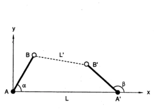
speeds. For convenience of discussion we set

up a Cartesian coordinate system as shown in

Fig. 3, where $A$ and $A’$ are at the origin _$(0,0)$

and $(L, 0)$, respectively, and $\alpha$ and $\beta$ are the

an-gles that $AB$ and $A’B’$ make with the $x$-axis,

re-spectively. In this section, we assume $L’\leq L$

and $0\leq\alpha,\beta\leq 180^{\mathrm{O}}$, where $L=|AA’|$ and $L’=|BB’|$

.

Minor changes are needed in the following discussion for other cases.

counterclockwise, whose directions are $\alpha+$

$\pi/2$ and $\alpha-\pi/2$, respectively.

Figure 3: The setup for ALGI and ALG2.

3.1

Distributed

algorithms

ALGI

and

ALG2

In this section we introduce two distributed

al-gorithms ALGI and ALG2. ALGI is for the

case where the two robots’ maximum speeds are

known toboth robots, whileALG2 is for the

case

where neither robot knows the other robot’s

max-imum speed. In either algorithm we assume that

the robots’ current and goal positions are known

to both robots. (This assumption can be

expen-sive to realize in practice.)

Both algorithms are memoryless in the sense

that their output is afunction of the current state

(and is independent of the motions in the past).

Itis therefore sufficienttoview $A$ and $B$ of Fig. 3

as the robots’ current positions and specify how

the velocity vector is computed from $A,$ $B,$ $A’$

and $B’$

.

Algorithm ALGI

Both robots know the maximum speeds $v_{A}$ and

$v_{B}$ ofboth, as well as the positions $A,$ $B,$ $A’,$ $B’$,

and hence angles $\alpha,$ $\beta$ and their offset vectors $\vec{\mathrm{O}}_{A}$

and $0_{B}arrow$

.

$c_{1},$ $c_{2}$, and $s\geq 0$ are some constants.

Since both robots have the same information we explicitly describe the procedure for both.

Step 1: Let $e_{A}=L/v_{A}$ and $e_{B}=L’/v_{B}$

.

Let $t_{A}arrow$

and $t_{B}arrow$ be vectors directed from _$A$

to $A’$ and

from $B$ to $B’$, respectively, such that

$\bullet$ $|t_{A}^{\sim}|=1$ and $|t_{B}|arrow=(e_{B}/e_{A})^{c_{1}}$ if _{$e_{A}\geq$}

$e_{B}$, and

$\bullet$ $|t_{A}|arrow=(e_{A}/e_{B})^{c_{1}}$ and $|t_{B}^{\sim}|=1$ if _{$e_{A}<$}

$e_{B}$

.

Step 2: Let $r_{A}arrow$ and $r_{B}arrow$ be “rotational vectors”

of length $c_{2}(\beta-\alpha)$ that rotate the ladder

$\mathrm{S}\mathrm{t}\mathrm{e}\mathrm{p}3:arrow$ Scale the offset vectors as $\vec{h}_{A}=SO_{A}arrow$ and

$h_{B}=so_{B}arrow$

.

Step 4: $\vec{T}_{A}=t_{A}+rA+\vec{h}arrowarrow A$ and$\vec{T}_{B}=t_{B}+r_{B}arrowarrow+\vec{h}_{B}$

.

Step 5: Output velocity vector

$\bullet$ $\overline{v}_{A}=v_{A}\vec{T}_{A/\max\{1\vec{T}|}A,$$|\vec{T}_{B}|$

}

for robot

$A$, and

$\bullet$ $v_{B} arrow=v_{B}\vec{T}_{B}/\max\{|\vec{T}A|, |\vec{T}_{B}|\}$ for robot

$B$

.

In Step 1 ALGI tries to slow the robot that

would otherwise reach its goal sooner than the

other according to the estimates $e_{A}$ and $e_{B}$

.

The

constant $s$ used in Step 3 isa parameter

indicat-ing how a robot reacts to the offset.

Algorithm ALG2

The robots have all the information available in

ALGI, except robot $A$ does not know

$v_{B}$ and

robot $B$ does not know

$v_{A}$

.

We use additional

constants $v_{A}’$ and $v_{B}’$

.

Step 1: Robot $A$ runs ALGI using

$v_{A}$ and $v_{B}’$

in place of$v_{A}$ and $v_{B}$, respectively. Likewise

robot $B$ runs ALGI using $v_{A}’$ and $v_{B}$

.

Let

$\overline{v}_{A}^{f}$ and $\overline{v}_{B}^{\mathrm{v}}$ the velocity vectorsobtained.

Step 2: Output velocity vector

$\bullet$ _{$v_{A}arrow=\overline{v}_{A}’$} if $|\overline{v}_{A}’|$ _{$\leq v_{A}$}, and $v_{A}arrow=$

$v_{A}v_{A}\neg/|v_{A}|\neg$ otherwise, for robot $A$

.

$\bullet$ $\vec{v}_{B}=v_{B}^{\neg}$ if $|\vec{v}_{B}’|\leq v_{B}$, and $v_{B}arrow=$

$v_{B}v_{B}arrow/|\overline{v}_{B}^{l}|$ otherwise, for robot $B$

.

InALG2we use$v_{A}’$ and$v_{B}’$ asan estimate of

un-known $v_{A}$ and $v_{B}$, and the output ofALG2

coin-cides with that ofALGI if$v_{A}’\leq v_{A}$ and $v_{B}’\leq v_{B}$

.

We

assume

that $v_{A}’$ and $v_{B}’$ are constants

sup-plied to ALG2, since it is one ofour basic goals

to keep the algorithms memoryless (memoryless

algorithms can tolerate a finite number of

tran-sient errors). Itwould be interesting, however, to

modify ALG2so that the robots will choose

suit-able values for $v_{A}’$ and $v_{B}’$ based on their recent

Figure 4: ALGI for $k=1,$ $\alpha=30^{\mathrm{o}},$ $L=200$

.

Figure 5: ALGI for $k=1,$ $\alpha=30^{\mathrm{o}},$ $L=400$

.

3.2 Experimental

results

by

computer

simulation

Using the setup of Fig. 3 we evaluate the

per-formance of the algorithms in terms of the time

necessary for the robotsto reach their goals. The

length $\ell$ of the ladder is 100, and the radius of

the disks representing the robots is 10. We use

$v_{A}=1$ and $v_{B}=k$ (so $k$is the ratio of

$v_{B}$ to $v_{A}$),

andin the following discuss mainly the results for

the case $k\geq 1$

.

The parameters $c_{1},$$c_{2}$ and $s$ of

ALGI areset to 3, 0.5, and 0.1, respectively, that

have been found to work well when $v_{A}=v_{B}[1]$

.

Toreduce the number of instances to examine, we

experiment with only two values of $L,$ $L=200$

$(=2\ell)$ and 400 $(=4\ell)$, while changing $\alpha$ in the

rangefrom $0^{\mathrm{o}}$ to $90^{\mathrm{o}}$ and setting _{$\beta=180^{0}-\alpha$}

.

Fig. 4 and Fig. 5 show the motions generated by ALGI for $k=1$ and $\alpha=30^{\mathrm{O}}$, for $L=200$

and $L=400$, respectively. Fig. 6 and Fig. $7\mathrm{s}\mathrm{h}_{0}\mathrm{w}$

the same, for $k=3$ _{instead of 1. The finish times}

for $L=200$ are 205 $(k=1)$ and 201 $(k=3)$, and for $L=400$ they are 404 $(k=1)$ and 401

$(k=3)$

.

Note that in Fig. 6 and Fig. 7 robot $B$

initially slows down considerably, allowing robot

$A$to rotate morequickly than in Fig.4and Fig. 5.

Fig. 8 and Fig. 9 show the finish times for $k=$

$1,2,3,4$and 5, for$L=200$ and 400, respectively.

Figure 6: ALGI for $k=3,$ $\alpha=30^{\mathrm{o}},$ $L=200$

.

Figure 7: ALGI for $k=3,$ $\alpha=30^{\mathrm{o}},$ $L=400$

.

Figure 8: Finish times of ALGI for $k=1,2,3,4$

Figure 11: ALGI with$k=1/3,$$\alpha=30^{\mathrm{o}},$$L=200$

.

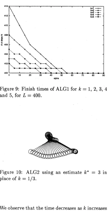
Figure9: Finish times ofALGI for $k=1,2,3,4$

and 5, for $L=400$

.

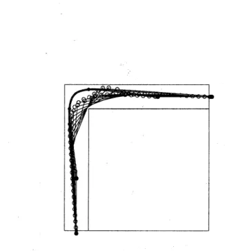
Figure 10: ALG2 using an estimate $k^{*}=3$ in

place of$k=1/3$

.

Weobservethat the time decreases as $k$increases

when $\alpha\leq 60^{\mathrm{o}}$

.

This phenomenon is quitenatural,

since smaller $\alpha$ implies more necessary rotation,

andlarger$k$ causes $B$ toslow down, thus allowing

$A$ to rotate more quickly.

Fig. 10 shows a motion generated by ALG2 for

$k=1/3,$ $\alpha=30^{\mathrm{o}}$ and $L=200$, where (for

sim-plicity) both robots use an estimate of$k^{*}=3$ in

place of the unknown $k$

.

(The estimates of $k$ by

$A$ and $B$ may differ in real situations.) Note that

the robots successfully complete the task even

though their estimate $k^{*}$ is not at all close to

ac-tual $k$

.

However, the large discrepancy between

$k^{*}$ and $k$ has resulted in a noticeable decline in

the performance in terms of the finish time –

the finish time ofALG2 in Fig. 10 is almost 28%

larger than that ofALGI in Fig. 11 for the same

instance.

4

Corridor with

a

Corner

The distributed approach works well also for the

case in which the robots must go through a 90

degree corner in a corridor avoiding both

robot-to-wall and $1\mathrm{a}\mathrm{d}\mathrm{d}\mathrm{e}\mathrm{r}- \mathrm{t}_{0^{-\mathrm{W}}}\mathrm{a}\mathrm{l}1$ collision. The motion

shown in Fig. 12 has been obtained by an

algo-rithm that is similar in spirit to the ones

pre-sented in the preceding section, with an

addi-tional step in which each robotcomputes a target

path through the corner before starting the

mo-tion. During the motion each robot attempts to

move along the path while adjusting its positions

based on both the $\mathrm{m}\mathrm{o}\mathrm{t}!\mathrm{o}\mathrm{n}$ of the other robot

ob-served through the force sensor and the need to

preventcollision. We assume that the robots can

detect how close they and the ladder are to the

walls, from their positions and the geometry of the workspace.

While the robots in the preceding section are

assumed to be identical in all aspects other than

their maximum speed, in this section we assume

that they may differ in a number of other

charac-teristics as well –(i) selection ofa path through

the corner (in, middle or out), (ii) the maximum

speed (high or low), (iii) adherence to the

in-tended path (high or low), and (iv) reaction to

the motion of the other robot (high, low, or

nonlin-ear). These variations result in atotal of36

differ-ent types of robots from which twoarechosen to

carry outthetask. Weassumethat the robots do

not know the characteristics of the other robot.

First, robot $R$ generates a path $P$ through the

corner as aKochanek-Bartels spline [6] that

trav-els either close to the inner walls of the corner

(in), close to the outer walls of the corner (out),

or somewhere in between the two (middle).

deter-Figure 12: Motion through a cornergenerated by

ALG3.

The robotsstart atthe bottom of the

fig-ure and makes a right turn. The intended paths

of the robots

are

shown in small circles.

mined by the following algorithm ALG3 that $R$

usesto computeits velocity vector. Itisassumed

that the offset$|\mathit{0}\urcorner$ can beaslarge as thethe radius

10 of the disk representing $R$

.

Algorithm ALG3

Step 1: $\vec{u}=(1/10)(\tilde{g}+f(\overline{o})+c\gamma$, where

$\bullet$ $\vec{g}$is avector of size 10directedfrom the

center of $R$toward the “current target

position”,

$\bullet$ $o\mathrm{i}arrow \mathrm{s}$the offset vector and _$f$is afunction

that converts$\vec{o}\mathrm{i}\mathrm{n}\mathrm{t}\mathrm{o}$ anothervectorsuch

that$|f(\vec{O})|\leq 10$ (seedetails bel$o\mathrm{w}$),and

$\bullet$ $carrow$ is a suitable “correction vector”

needed to prevent collision. (We omit

the details of$c$)

$\sim$

.

The factor 1/10 effectively reduces the sizes

of$\vec{g}$and $f(\vec{o})$ to within 1.

Step 2: $\tilde{w}=\vec{u}$if $|\tilde{u}|\leq 1$, and $\vec{w}=\vec{u}/|\vec{u}|$ if $|\vec{u}|>$

$1$

.

That is, $\vec{w}$ is the result of “clamping”

vector $\vec{u}$at length 1 so that

$|\vec{w}|\leq 1$

.

Step 3: Output the velocity vector $\vec{v}=V\vec{w}$,

where $V$ is the maximum speed of$R$

.

In our experiments the maximum speed $V$ of

$R$ can be either 2 (high) or 1 (low).

A robot with high adherence attempts to

re-turn to $P$ more quickly than one with low

ad-herence when it deviates from $P$

.

We control the

ad herence of$R$ bychoosingvector$\vec{g}$in Step 1

ap-propriately: If adherence is high then the “current

target position” (at which $\vec{g}$ is aimed) is chosen

to be a point on $P$ relatively close to the robot’s

current location. If adherence is low then $\tilde{g}$ is

di-rected toward a point on $P$ that is farther away.

(We omit the details of how such points are

ac-tually chosen in our experiments.)

Function $f$of Step 1 determines how$R$ reacts

tothe motion of the other robot observed through

$\tilde{o}$

.

We use the following three variations.

1. high: $f(\vec{o})=\tilde{o}$

.

The robot is highly sensitive

to $\mathit{0}arrow$

.

2. low: $f(\mathit{0})arrow=0.5\tilde{o}$

.

The robot’s sensitivity is

low.

3. nonlinear: $f(\vec{o})$ equals the zero vector $0arrow \mathrm{i}\mathrm{f}$

$|\mathit{0}\neg\leq 5$, and $2_{\mathit{0}^{\wedge}-}\tilde{O}/|\mathit{0}\neg$ if $|\mathit{0}\neg>5$

.

The robot

reacts to $o\mathrm{o}\mathrm{n}\mathrm{l}arrow \mathrm{y}$ after its magnitude exceeds

5.

Note that $|f(\vec{O})|\leq|\mathit{0}\neg\leq 10$ holds in all three

cases.

The motion shown in Fig. 12 is obtained by

ALG3 where both robots use the same out path

and has the same low adherence. The robot in

front has high maximum speed and high reac-tion $(f)$, while the other robot has low maximum

speed and nonlinear reaction.

To evaluate ALG3 we randomly generate 100

pairs of robots from the pool of 36 robots and

ex-amine the probability that the task is completed

successfully (a motion is considered unsuccessful

ifthe offset exceeds 10). Thewidth of the corridor

is 200 and the ladder length $\ell$varies between 400

and 480. (The robots always fail when $\ell=490.$)

Thesuccess rate decreases from 100% for$\ell=400$

to 75% for $\ell=480$ if both robots are _allowed

to choose a path that is either in, middle or out,

while the rate increasesto 100% for$\ell=480$if

nei-ther is allowed to choose an in path. However, if

we allow the robots’ adherence to be even higher

(than high), then the rate drops again to 57% for

$\ell=480$ even without in paths. The reader is

analysis of the effect of these parameters to the

overali

perfOrmanC.

$\mathrm{e}$

.

5

Concluding Remarks

We have presented three distributed algorithms

for two robots carrying a ladder under various

conditions, and evaluated their performance

us-ing computer simulation. We arecurrently

work-ingon a detailed analysis ofALG3.

References

[1] Y. Asahiro, H. Asama, S. Fujita, I. Suzuki

and M. Yamashita, “Distributed algorithms

for carrying a ladder by omnidirectional

robots in near optimal $\mathrm{t}\mathrm{i}\mathrm{m}\mathrm{e}_{7}$” in Sensor

Based Intelligent Robots, H.I. Christensen,

H. Bunke and H. Noltemeier, Eds., Lecture

Notes in Artificial Intelligence, Vol. 1724,

Springer Verlag, Heidelberg, Germany, pp.

240-254, December 1999.

[7] Y. Kawauchi, M. Inaba and T. Fukuda,

“A principle ofdistiributed decision making

ofcellular robotic system (CEBOT),” Proc.

IEEE Int.

_Conf.

on Robotics and

Automa-tion, pp. 833-838, 1993.

[8] K. Kosuge and T. Oosumi, “Decentralized

control of multiple robots handling and

ob-jects,” Proc. $IEEE/RSJ$Int.

_Conf.

on

Intel-ligent Robots and Systems, 556-561 (1996).

[9] N. Miyata, J. Ota, Y. Aiyama, J. Sasaki,

and T. Arai, “Cooperative transport

sys-tem with regrasping car-like mobile robots,”

Proc. $IEEE/RSJ$ Int.

_Conf.

on Intelligent

$Roh)ts$ _{and Systems, pp. 1754-1761,} 1997.

[10] S. Nagafuji, Y. Asahiro, M. Yamashita and

I. Suzuki, “Time-optimal motion of two

heterogeneous robots carrying a large

ob-ject,” in Proceedings

_of

1999 Joint

Confer-ence

_of

Electrical and Electronics Engineers

of

Kyushu (in Japanese), page 742, October

1999.

[2] Y. Asahiro, H. Asama, I. Suzuki and M.

Ya-mashita, “Improvement of distributed

con-trol algorithms for robots carrying an

ob-ject,” in Proceedings

_of

1999 IEEE

Interna-tional

_Conference

on$SystemS_{f}$ Man and

Cy-bernetics, pp. VI 608-613, October 1999.

[3] H. Asama, M. Sato, L. Bogoni, H. Kaetsu,

A. Matsumoto, and I. Endo, “Development

of an omni-directional mobile robot with 3

DOF decoupling drive mechanism,” Proc.

IEEE Int.

_Conf.

on Robotics and

Automa-tion, pp. 1925-1930, 1995.

[11] J. Pearl, Heuristics - Intelligent Search

Strategies

_for

Computer Problem Solving,

Addison-Wesley, 1984.

[12] Z. Wang, E. Nakano and T. Matsukawa,

“Realizing cooperative object manipulation

using multiplebehavior-based robots,” Proc.

$IEEE/RSJ$ Int.

_Conf.

on Intelligent Robots

and Systems, pp. 310-317, 1996.

[4] E.C.-H. Chang, “Distributed motion

coor-dination of two robots carrying a ladder

in a $\mathrm{c}\mathrm{o}\mathrm{r}\mathrm{r}\mathrm{i}\mathrm{d}\mathrm{o}\mathrm{r}_{7}$” MS Thesis, EECS

Depart-ment, University of Wisconsin-Milwaukee,

in preparation.

[5] Z. Chen, I. Suzuki, and M. Yamashita,

“Time optimal motion of two robots carrying

a ladder under a velocity constraint,” IEEE

Trans. Robotics and Automation 13, 5, pp.

721-729, 1997.

[6] D. Hearn and M.P. Baker, Computer