流体シミュレーションによる炎の形状制御

全文

(1)Vol.2014-CG-155 No.8 2014/6/28. 情報処理学会研究報告 IPSJ SIG Technical Report. 流体シミュレーションによる炎の形状制御水谷圭佑†1. 佐藤周平†1. 土橋宜典†1. 山本強†1. 本論文では流体シミュレーションに基づく炎のアニメーションの運動制御手法を提案する．運動制御には，従来研究である流体シミュレーションに基づく煙の制御手法を用いる．しかし，炎のシミュレーションでは炎の高い温度による強い浮力が生じるため，煙に対する手法をそのまま炎に対して用いるだけでは目標形状に制御することが難しい．本研究ではこの問題を解決するため，ユーザにより指定された目標形状と炎の形状との差分から局所的に制御力を自動で調節する．これにより，炎を目標形状に制御することが可能となる．. Controllable Simulation of Fire based on Computational fluid Dynamics KEISUKE MIZUTANI†1 SYUHEI SATO†1 YOSHINORI DOBASHI†1 TSUYOSHI YAMAMOTO†1 In this paper we present a method for controlling fire simulation based on computational fluid dynamics. Our method applies a previous method for controlling smoke simulation to fire simulation. However, controlling fire simulation is difficult when using the previous method, because in the fire simulation, strong buoyancy forces caused by high-temperature of fire are arisen. To address this problem, our method locally adjusts a parameter of control forces in the previous method using a difference between the user-specified target shape and the simulated fire shape. Our method can control the fire into an arbitrary shape specified by the user.. 1. まえがきコンピュータグラフィックス（CG）において流体解析を利用した炎や水の動きを計算する研究が盛んに行われている．映画やコンピュータゲームなどでは煙，炎，水などが様々な形状として表現される映像が利用されることがある．このような映像の写実性を追求するには，流体力学に基づ. [6]を応用して炎の形状をコントロールする．加わえて，目標形状と炎の形状の差分から局所的に制御力を調節する．提案手法により，ユーザが指定した形状に制御された炎のシミュレーションが可能である．. 2. 提案手法提案手法では，炎の流体シミュレーションと Fattal らの. いた自然現象の動きをコントロールすることが有効であり，. 手法を組み合わせることで，指定された所望の形状の炎の. 流体シミュレーションの制御のための研究[1][2][3]が提案. 生成を行う．動きのコントロールは，炎が目標とする形状. されている．従来研究では，煙や水の動きを外力を用いて. となるような外力を加えることで行う．外力として，Fattal. 制御している．しかしながら，炎のシミュレーションの制. らの手法の driving force を利用する．図 1 に提案手法の概. 御は，煙や水に対する従来手法を適用するだけでは難しい．. 要を示す．まず，ユーザにより入力された目標形状から目. 一般的に，炎は浮力により燃え上がっており，加えてその. 標密度を計算する．次に，計算された目標密度の勾配を用. 強い浮力が従来手法を用いた制御力を妨げてしまう．. いて driving force を求め，炎のシミュレーションに適用す. 炎の形状をコントロールする方法に関する研究[4][5]が. る．. いくつか提案されている．しかしながら，どちらの手法も. しかし，煙に対する従来手法を炎に用いた場合，煙には. 流体シミュレーションに基づくものではない．炎のリアル. ない強い浮力の影響により，形状制御が難しくなる．その. な映像は，流体シミュレーションを用いて作成される場合. ため，形状を考慮した局所的な driving force の係数の調節. が多い．また，ユーザが意図した任意形状の炎のアニメー. を行う．本手法では，2.3 節で後述する，炎の形状と目標. ションを容易に生成できることは，映像表現の一つとして. 形状の差分を用いて計算される累積分布を用いて，driving. 有用である．そのため，より現実の動きに近いアニメーシ. force の係数を調節する．炎の形状は炎の温度分布を二値化. ョンを作るために，流体シミュレーションを制御すること. することにより得る．以下でこの手法について詳しく説明. が有効である．. を行う．. 本研究では，流体力学に基づいた炎の動きの制御を行う．ユーザが入力した目標形状をもとに，Fattal らによる手法 †1 北海道大学 Hokkaido University. ⓒ 2014 Information Processing Society of Japan. 2.1.. 炎のシミュレーション. 本論文では，以下で説明する簡易モデルによりシミュレーションを行う．まず，図 2 のようにシミュレーション空間を格子で分割し，各格子点において速度および温度を割. 1.

(2) Vol.2014-CG-155 No.8 2014/6/28. 情報処理学会研究報告 IPSJ SIG Technical Report. 図 2：シミュレーション空間れた位置の密度を引き寄せるために目標密度 ρ~ * で割るこ. 図 1：提案手法の概要. とで規格化を行う．りつける．また，シミュレーション空間の下端中央に炎を発生させる領域(ソース)を配置する．毎ステップの処理は以下のようになる．配置したソースに鉛直上向きの速度と温度を与えることで炎の発生を疑似的に表現する．その後，シミュレーション空間内の速度場および温度場を文献[7] の方法を応用して計算することで炎をシミュレーションする． 2.2.. 2.3.. 制御力の調節. 炎は目標形状に沿って発展するため，目標密度から離れた位置では driving force の効果はほぼない．加えて，炎には強い浮力があるため，熱源の温度などの影響により，炎が目標形状を越えてしまうことがある．これを防ぐため，シミュレーション空間全体で一定であった driving force の係数 νf の代わりに，各格子点でその大きさを変化させた係数 νf (x)を用いる．これは図 4 に示す累積分布を計算するこ. 流体の運動制御. 炎の運動制御を行う driving force は，図 3 に示すように，. とにより得られ，以下の式で与えられる．. 指定した目標密度に炎を一致させるような流れを生み出す外力である．この項は流体運動の速度場を表現する N-S 方. ν (f n ) (x) = k f ρcu( n ) (x)ν (f n−1) (x) ,. (2). 程式に外力項として付加され，目標密度分布を用いて各タイムステップにおいて発展していく密度分布を元に計算される．以下にその構成過程を示す．driving force は以下の式. ここで kf はユーザにより指定される制御係数，ρcu(x)は差分累積分布である．これは以下の式であらわされる．. で表される．. ∇ρ~* ~ F ( ρ , ρ ) = ν f ρ ~* , ρ *. (1). ρ は各タイムステップでの密度，ρ＊はユーザが設定する目標密度を表す．νｆは driving force の大きさを調節するための係数である． ρ~ および ρ~ * は，それぞれ，ρ および ρ*に対して，ガウス関数との畳み込みを行ったものである．目標密度の勾配∇ρ＊は目標密度の値が大きい方向を常に指す．そのため，F は目標密度方向への流れを生み出すことになる．ここで，F = 0 となる場所ができてしまうことを避けるために，∇ρ＊ではなく∇ ρ~ * を用いる．次に， driving force が適用される位置を密度 ρ が存在する範囲の周辺のみに限定するため，F を ρ~ に比例させる．また，目標密度から離. ⓒ 2014 Information Processing Society of Japan. ρ cu( n ) (x) = {ρ bi (x) − ρ * (x)} + kc ρ cu( n −1) (x) , . ρ bi (x) =  . 1 (T (x) ≥ Tth ) 0 (T (x) < Tth ). (3) (4). ,. ここで，kc は累積係数，ρbi(x)は温度を閾値として設定し，温度を二値化することで得られる炎の二値分布である．ここで，Tth は実験的に決定した温度の閾値である．ρbi(x) ρ*(x)が負の場合は０を設定し，累積係数は０から１までの値を設定する．driving force の係数は累積分布に比例し，kc の値を大きくすると，差分累積が大きい場所の driving force がより強くなる．これにより，炎が目標形状を越えて移動してしまうことを防ぐ．. 2.

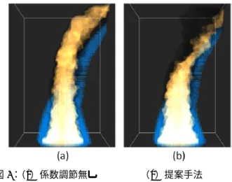
(3) Vol.2014-CG-155 No.8 2014/6/28. 情報処理学会研究報告 IPSJ SIG Technical Report. 図 3：driving force による外力図 4：差分累積分布の生成過程. 3. 実験結果提案手法により制御された炎のシミュレーション結果を図 5 に示す．目標形状は Y 字形状を設定し，シミュレーション空間の格子数は 64×64×96 である．実装環境は CPU：. Intel Core i7 3.50GHz，GPU：NVIDIA GeForce GTX 780，メモリ：8.00GB，グラフィックス API：OpenGL である．累積係数 kc は 0.95，閾値温度 Tth は実験的に決定した 0.4 に設定している．提案手法により driving force の係数が自動的に調節され. 図 5：Y 字形状に制御された炎のシミュレーション結果. た例を図 6 に示す．（a）が提案手法を用いない場合で，（ b）が提案手法である．目標形状は青色の点で示している．図に示すように，（b）の炎の形状の方が（a）の炎の形状よりも目標形状により近いことが確認できる．. 4. まとめ本論文では，流体解析に基づいた炎の動きの制御手法を提案した．提案手法では，炎の形状と目標形状との差分の累積分布を計算することにより，driving force の係数を局所的に調節した．これにより，炎がユーザの指定した形状に沿うアニメーションの生成が可能となった．本手法では driving force のみを用いて炎のシミュレーションを制御した．今後の課題として，より複雑な形状への. 図 6：（a）係数調節無し. （b）提案手法. 制御のために浮力を自動調節することなどが挙げられる．. Alfred R. Fuller, Hari Krishnan, Karim Mahrous, Bernd Hamann, and Kenneth I. Joy. Real-time procedural volumetric fire. In Proceedings of the 2007 Symposium on Interactive 3D Graphics and Games, I3D '07, pp. 175-180. 6) R. Fattal and D. Lischinski, Target-driven smoke animation, In Proceeding of ACM SIGGRAPH 2004, pp. 441-448. 7) D. Q. Nguyen, R. Fedkiw, H. W. Jensen 2002, Physically Based Modeling and Animation of Fire, In Proceeding of ACM SIGGRAPH 2002, pp. 721-728.. 5). 参考文献 Jeong-MoHong and Chang-Hun Kim. Controlling fluid animation with geometric potential. In Computer Animation and Virtual Worlds (CASA 2004), Vol. 24, pp. 140-164, 2005. 2) Anitoine McNamara, Adrien Treuille, Zoran Popovic’, and Jos Stam. Fluid control using the adjoint method. In ACM Transactions on Graphics, pp. 449-456, 2004. 3) Lin Shi and Yizhou Yu. Taming liquids for rapidly changing targets. In ACM SIGGRAPH/Eurographics Symposium on Computer Animation, pp. 229-236, 2005. 4) Arnauld Lamorlette and Nick Foster. Structural modeling of flames for a production environment. In Procedings of the 29th Annual Conference on Computer Graphics and Interactive Techniques, SIGGRAPH '02, pp. 729-735. 1). ⓒ 2014 Information Processing Society of Japan. 3.

(4)