近畿大学学術情報リポジトリ

全文

(1)Mem. School. B.O.S.T. Kinki University No.4: 23--45 (1998). 23. Design and Development of a Binary Filter for Image Differentiation (No.2) Sadahiko Nagae Abstract In the present study, to realize a filter in the optical differentiation with a binary configuration, in succession to the previous report, the author determined a concrete procedure and dimensions for its fabrication, and showed how to measure intraplane distribution of strain gradient of a flat plate that depends only on the phase distribution as an experiment in the practical application. It was confirmed as the result that the filter fabricated with digital procedure could give a good outcome similarly to the analog filter. The author also attempted, on the other hand, the optical differentiation of images by changing only amplitude distribution while keeping phase distribution unchanged. In this case, too, it was confirmed that the digital filter could give correct output images similarly to the analog filter. At the present moment, overall processing time is longer than the present digital computer aided processing because the recording of output images has relied eventually on the analog processing based on the past photographic development. If a device fully capable of digital processing is developed soon or later, an optical operation system that allows real-time on-line processing seems to become possible. Introduction. When an object is illuminated with a monochromatic light to make its image, in general, the imaging optical system is called the double diffraction optical system. All theories and experiments in the present study are provided as conducted with this double diffraction optical system and with a coherent light source such as laser light. Well, if the author considers the imaging optical system from the standpoint of transmission theory, it gets easier in treatment and often shows effective functions for various problems. In a coherently illuminated imaging system, the optical system can be regarded as a kind of linear transmission system when we consider amplitude distribution of the wave front that passed through the object as the input and that at the image plane as the output in comparison of time axis in the transmission system with spatial axis of the optical system. Thus, a variety of mathematical operations become possible between the amplitude transmittance distribution of the object and that of the image when a spatial filter is inserted, for actively varying characteristics of this transmission system, on the spectral plane of the optical system, namely on Fraunhofer diffraction plane at the back focal plane just behind the object. In the first report 1), we described, as one of this operation, on the principle of optical differentiation, a method of designing the optical differential filter necessary for it, .and evaluation of the filter. Then in the present paper, we show Department of Electronic Systems and Information Engineering, Kinki University, Wakayama 649-6493, Japan'.

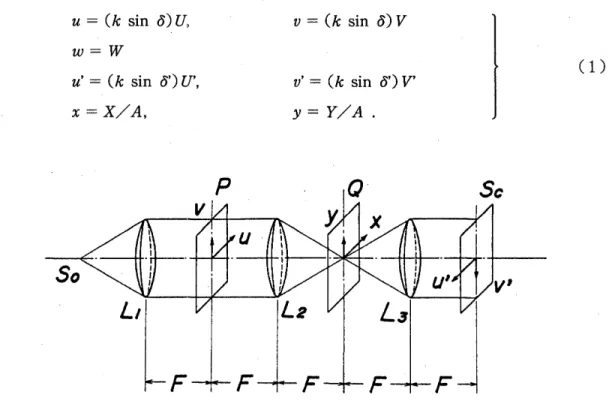
(2) 24. Memoirs of The School of B.O.S.T. of Kinki University No. 4 (1998). a concrete procedure of fabricating the binary filter and an example of more practical applications by Ineans of this image differential method. 1 • Principle. First of all, we describe here the principle of optical differentiation method to help comprehend the application example mentioned later.. 1 . 1 Double Diffraction Optical System Fig. 1 shows the imaging system and its coordinate system used in the present study. It is assumed that the optical system is entirely free from aberration and consideration is restricted to imaging of paraxial rays only. Accordingly, it is provided that isoplanatism has always held good. In the figure, (So) represents an ideal coherent light source; and (P), (Q) and (S) denote object, spectral and image planes, respectively. Collimator, condenser and projection lenses are denoted as (L I ), (L 2) and (L 3 ), respectively. It is also provided to employ coordinate conversion 2) of Eq. ( 1) to simplify comparison of object with image as mentioned later, to ease operation of Fourier conversion and to make treatment of equations dilnensionless for generalization. u = (k sin 0) U,. v = (k sin 0) V. w=W u'. = (k sin 0') U',. x = X/A,. ( 1) v' = (k sin 0') V' y = Y/A .. So. Fig. 1. Double diffraction optics and its coordinate system. Here, k = 27r/it is propagation constant and it denotes wavelength of the light source. Capital letters represent actual coordinates and give true geometrical lengths. A is radius of the projection lens, 0 is aperture angle of the combined.

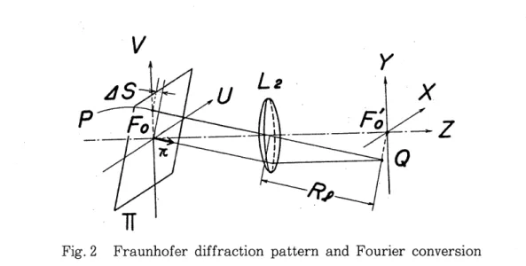
(3) 25. system of projection and condenser lenses, and 0' is that of the projection lens viewed from image side. The coordinate system of the object plane is denoted as (u, v), and that of the conjugate plane of light source with collimator and condenser lenses, namely of Fraunhofer diffraction plane, is as (x, y). Further, (u', v') shows coordinate system of the image plane and w is the sample coordinate along the light axis. Well, the imaging magnification of this optical system M is given as U' U. V' V. -=-=M. (2). and use of the conversion coordinate of Eq. ( 1) is convenient because the object and image correspond to each other at magnification of unity and calculation can be advanced in dimensionless as well. Now provided that feu, v) is denoted for distribution of complex amplitude transmittance possessed by an object structure, complex amplitude distribution of its diffraction pattern on Fraunhofer plane (x, y) is given with Fourier conversion of feu, v), namely o(x, y) = :F {feu, v)}. Similarly, complex amplitude distribution of the wave front on the image plane (u', v') is given by Fourier conversion of o(x, y), namely f'(u', v') = :F{o(x, y)}. Accordingly, because the condenser lens has such an aperture as to entirely pass all the wave front from the object and is free from aberration, amplitude distribution of the wave front on the image plane eventually becomes f'(u', v') oc feu, v) from Eqs. ( 1) and (2). Leaving detailed calculation for these in Section 1. 2, we point out here the fact that amplitude distribution * of the object (image of the object) same as in geometrical optics does appear on the image plane. When the imaging is conducted with two Fourier conversions, namely with two-fold diffraction, this imaging system is called the double diffraction system, and employed throughout this paper from now on. 1 .2 Fraunhofer Diffraction Pattern and Fourier Conversion In the previous figure, light wave that left the coherent point source (So) Passes through the collimator lens (L I ), and then forms a parallel plane wave to uniformly illuminate the object (T). It is shown here that amplitude distribution of a diffraction pattern on Fraunhofer diffraction plane (spectral plane) conjugate with the light source is given with Fourier conversion of amplitude transmission distribution of the light wave that passed through the object. In Fig. 2 , the object is placed on a plane (U, V) that contains the front focal point (F) or" the lens (L 2 ) and perpendicular to the optical axis (made agree with z axis). At this point, we represent complex structure of the object with the following equation: * *. feu,. V) = /o(U, V)· exp{jif>(U, V)} .. * Because coordinates. Cu', u') and Cu, u) have been taken in the opposite directions as shown in Fig. 1 . image of j'(u', u') has the shape inverted of the object, agreeing with imaging in geometrical optics. * * Transmittance of an object generally contains both of amplitude structure that brings decay in amplitude of the light wave and phase structure that gives variation in phase of the light wase due to thickness or refractive index. What expresses amplitude and phase at the same time as shown in Eq.C 3) is generally called as complex structure of the object.. ( 3).

(4) 26. Memoirs of The School of B.O.S. T. of Kinki University No.4 (1998). v. y. x --z. p. Q. IT Fig. 2. Fraunhofer diffraction pattern and Fourier conversion. Here, foe u, V) denotes amplitude transmittance distribution. Besides, ,p( U, V) is similarly a delay in phase caused by a change in thickness of the object or distribution of refractive index. When here is incidence of a parallel plane wave Eo . exp {j w r} with angular frequency wand amplitude Eo from the collimator lens (L 1), amplitude distribution just after passing through the object becomes. feu,. V, r) = Eofo(U, V)· expj{wr+,p(U, V)} .. (4). It is provided that the light wave that advances in the direction of unit vector -; in those passed through an object is condensed upon the diffraction plane (X, Y) through the lens (L 2 ). It is attempted at this time to calculate how amplitude distribution of the diffraction pattern is expressed. If denoting direction cosines of the unit vector -; as l, m and n, respectively, the plane II perpendicular to -; is expressed as follows: lU+mV+nz = 0 .. (5). Provided that LlS denotes the distance from a point P( U, V) on the object through the center of lens (L 2 ) until crossing the plane (II), it is expressed as follows: LlS. = lU+mV .. (6). By the way, the light wave (8) passing through the plane (II) contains the back focal point (F'o) of the lens (L 2 ) and focuses at a point Q(X, Y) on a plane (X, Y) perpendicular to the light axis, the phase distribution ,pn of the wave (8) on the plane (II) is. ,pn = ,p( u,. V) - k(ZU +m V) .. ( 7).

(5) 27. Besides, when denoting focal length of the lens (L 2 ) as F, and distance from the lens center to the point Q as R z , direction cosines become. 1 = X/R z,. m = Y/R z,. n = F/Rz. (8). as will be clear from the figure. Thus from Eqs.7 and 8 the phase at the point Q becomes. if>.1 = if> ( U, V) - k ; (UX + VY) - k L1. (i,. Y) .. (9). Here, L1 (X, Y) / F represents the light path length from the origin Fo of the plane (U, V) to the point Q(X, Y), and k is propagation constant that converts the light path length into the phase, being given with Eq.( 1). Now, amplitude distribution of the light wave at a point (X, Y) on the diffraction plane (X, Y) becomes o(X, Y, r). =. J. Eo' exp{j w r} i:fo(U, V)· expj{if>(U, V) -k ; (UX+VY)-k L1(i Y)}dUdV .. (10). In the optical system used in the present study, L1 (X, Y) is considered to be kept unchanged because the angle between the optical axis and light beam is small and we have determined to deal only with the paraxial ray3. 4). Because n =. 1 holds good in this case Eq (10) becomes as follows: o(X, Y). =. Co. Ji : fo(U,. V). 0. exp{j if>(U, V)} (11). oexp{-j ; (UX+VY)}dUdV .. Here, the temporal term is omitted and constant terms not relating to integration are assembled into Co. By the way, from Eq.( 1) A u=ko-U F. A v=ko-V F. Y y=A. X x=-. A. ). (12). is given if provided as sin 0 =. tan 0 = A/F. When substituting Eq. (12) into Eq. (11) and using Eq. (3) as well, we eventually obtain o(x, y) =. C'oJi:f(u,. v). 0. exp{ -j(ux+vy)}dudv. (13).

(6) 28. Memoirs of The School of B.O.S. T. of Kinki University No. 4 (1998). from which it is found that o(x, y), a function of x and y, IS gIven as Fourier conversion of I(u, v), a function of u and v. It was proved therefore that amplitude distribution of the light wave on Fra.unhofer diffraction plane conjugate with the light source is nothing but Fourier conversion of amplitude distribution of the wave front that passed through the object. Here, this Fourier conversion may be simply called as spectrum of the object and Fraunhofer diffraction plane as the spectral plane. Similarly, amplitude distribution of the wave front on the object plane is given with Fourier conversion of amplitude distribution of the spectral plane. Accordingly, amplitude distribution of the wave front on the image plane is also given with Fourier conversion * of alnplitude distribution of the spectral plane, namely I'(u', v') =. C~.ri : o(x,. y)exp{j(xu'+yv')}dxdy. (14). so from Eqs.(13) and (14), I'(u', v') -- I(u, v) holds good. By the way, intensity distribution of the image becomes leu', v') = I'(u', v') ·I;*(u', v'). (15). where, the sign * denotes complex conjugate. 1 .3 Spatial Filter and Optical Differentiation Provided the light wave shows a change of A (u, v) in amplitude and a difference of E,/u, v) when it passes through an object, complex structure of the object I(u, v) is given with the following equation: I(u, v) = A (u, v) . expj kE,d(u, v) .. (16). Here, when distribution of refractive index of the object is denoted as nc(u, v), distribution of its thickness as g(u, v), and refractive index of air is 1,. E,d(u, v) becomes as follows:. (17) Now, amplitude distribution of Fraunhofer diffraction pattern of this object IS given by o(x, y) =. J. i:/(u, v) . exp{ -j(xu+yv)}dudu .. (18). from previous Eq. (13). Further, amplitude transmittance distribution I'(u', v') of the image plane (namely, object plane) becomes I'(u', v') = * However, directions of. Ji:. o(x, y) . exp {j(xu'+yv')} dxdy .. u' and v' are opposite to those of x and y as shown in Fig. 1 .. (19).

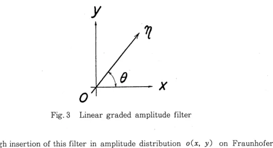
(7) 29. by Fourier conversion of o(x, y). Thus, partial differentiation of both sides of this equation with u', for instance, gives a{f'(u' v')} au: =. JJoo-ooj x . o(x,. y) . exp {j(xu'+yv')} dxdy. (20). == fI (u', v') . Accordingly, comparison of this Eq. (19) with Eq. (20) allows us to say as follows: It shows that amplitude distribution of the image obtained through its Fourier conversion becomes partial differentiation of the original amplitude distribution using u when we change amplitude distribution (underlined) of the object on Fraunhofer diffraction plane by inserting on the plane a spatial filter with amplitude transmittance distribution in proportion to x. In general, linear graded amplitude filters are shown with sex, y) = sex cos (). + y sin ()). (21). where, s is a constant denoting gradient of the filter, and the direction for the maximum gradient is expressed with T] as shown in Fig. 3 .. y. x. o Fig. 3. Linear graded amplitude filter. Trough insertion of this filter in amplitude distribution diffraction plane, its Fourier conversion becomes fl'(u', v') = js { of (~~, v') cos (). +. of (;;,. 0. (x, y). v') sin ()} .. on Fraunhofer. (22). Because the quantity enclosed with { } on the right side 'eventually becomes equal to af'(u', v') / aT], it is found that partial differentiation of amplitude distribution of the object in arbitrary direction can be obtained with direction of the filter..

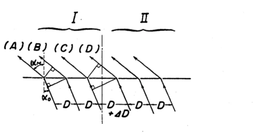
(8) 30. Memoirs of The School of B.O.S.T. of Kinki University No. 4 (1998). 1 .4 Configuration of Dlifferentiation Filter and Optical System The filter of Eq. ( 1) is opaque for x = 0, and its amplitude transmittance S increases with Ixl. However, S < in the range of x < 0, . which means negative transmittance being impossible in reality. Thus, it is necessary to separately fabricate an amplitude filter ISA I of IS(x) I and a phase filter Sp with which the phase delays by 7l for x < in comparison with x > 0, and to combine these two. Because this "combined filter", so to speak, has already been reported 5), we intend here to realize a differential filter by means of binary method. When we divide an opaque plate into surface elements with equal area, make a rectangular aperture (cell) on each of them, and insert this on the diffraction plane, amplitude distribution of the light wave passing through this varies with area of the cell, and phase distribution depends on relative position of each cell. Eventually, the light wave through this is affected by both amplitude and phase. Lohmann et al. 6 - 8 ) attem.pted design of Matched filter by making use of this principle. Because design of this filter requires complicate numerical calculation in general, we need help by a computer-aided automatic drafting machine and an X - Y plotter. In the differential filter, however, design is relatively simple. First of all, we describe on the control of phase. Variation in the amplitude of the light wave immediately after passing S (X) = sX is regarded, from the original light wave exp j (JJ T, as sX . exp j(WT+O). Here, 0 denotes phase and W shows angular frequency of the light wave. By the way, in the range of X < 0, when phase delay cp is given to 0 by 0' = (2N -1) 7l. °. °. cp = sX· expj{un+(2N-1)71+0} (23) = -s)[ . expj(wT+O). holds and the light wave reverses its phase. Thus we describe here a method in which diffraction lattices are divided into two groups and phase delay is given by shifting pitch of one group from the other.. [. fA). (B~. ~>(. II. (e) (D)!. : I. Fig. 4. Phase delay with lattice.

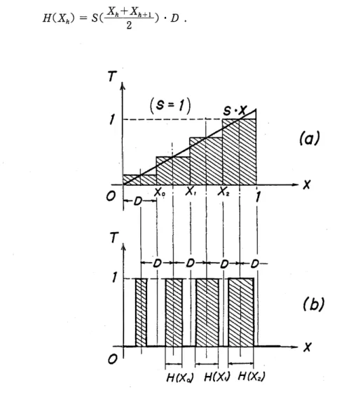
(9) 31. Let us consider diffraction lattice with pitch D as shown in Fig.4. Provided the pitch changed at a place by LiD, when the light wave incident at angle a o on this diffraction lattice passed through I and II lattice groups, a leap of phase difference is produced between each group of the light wave. We calculate such a value of LID that this leap of phase difference becomes 7[. Provided in the same figure that the light path difference between the light (A) and (B) is denoted as L M' and similarly that between (C) and ( D) as L'u, the optical plrase difference shall be intended intend to produce the leap of (24). When denoting the diffraction angle as aM' the difference in the path differences between { (A), (B) } and { (C) , ( D) } is LiL =. I(sin. = LID .. a M - sin ao) . D- (sin a M - sin ao) (D+ LID) I. I(sin. (25). a M - sin ao) I. from the figure. Provided that the order of diffraction spectrum becomes LlL = N'A • L1D. IS. N, Eq. (25). (26). D. so the phase delay q;M is given as m. =. k . LlL = 27[N· LiD. 'YM. D. (27). When inserting this diffraction lattice into the light wave as a filter, a leap in the phase change by q;M appears between iight waves through I and diffraction groups. Thus, when the leap in phase change by, 7[ is produced in the + 1 order diffracted light with N = 1, LlD=R 2. (28). is led from Eq. (27). This gives the phase filter Sp in question. Then the author describes on how to control the amplitude by means of the same diffraction lattice. Amplitude distribution of the light wave that passed through a cell is restricted with the cell area. Accordingly, a prescribed amplitude distribution can be obtained by changing each cell size stepwise. As shown in Fig. 5 (a) first, amplitude transmittance sX of the filter is approximated with folded line of hatched rectangles. The interval from X = 0 to 1 is equally divided with pitch D under S = 1. And the total sum of rectangular areas is made equal to integral of S(X) = X from X = 0 to 1. Because the amplitude transmittance is regarded fixed in each interval D, aperture with area proportional to this value.

(10) 32. Memoirs of The School of B.O.S.T. of Kinki University No. 4 (1998). was realized by changing the breadth in X direction as shown in Fig. 5 (b). In the figure, hatched areas are apertures with transmittance of unity, and the thick solid line shows distribution of transmittance (T). In this case, we approximately materialized amplitude distribution of the light wave that passed through the amplitude filter ISA I from. (29). T. (s = 1) 1 (a). T 1 (b). o Fig. 5. Approximation of amplitude filter I SA I. In order to give a change in addition, it is necessary from Eq. (28) to shift the pitch of diffraction lattice by D/2 at the origin. In this way, we realized a binary filter with which amplitude and phase of the light wave can simultaneously be controlled. Fig. 6 shows an example of binary filters using photographic film. For its fabrication, we used a microplotter (made by Mutoh Industry) to manually draw a pattern 100 times the original size on a white paper. By demagnifying this twice by means of photographic camera, we obtained the binary filter with the prescribed dimension (accuracy of 0.2 11m)..

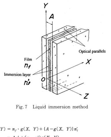
(11) 33. Fig. 6. An example of binary filter. When this filter is inserted on the diffraction plane of Fig. 1 to observe image of the object, only the diffracted light with odd order (N = 1, in the present case) gives differential image and that with even order including zero is imaged as noise. Because of this, separation of the image is necessary. Thus, denoting size of the object as L and focal length of the projection lens as F, the image size L' is given with the following formula 9): L' ~. INI . F. . A. / L .. (30). As 35 mm photographic film is often used as the object conventionally, we conversely consider boundary of the pitch D required to separate this from U' = L = 35 mm. Provided that the light source is laser light with wavelength of 632.8 nm· and focal length of the projection lens in Fig. 1 is 500 mm, D = 10,um is obtained to separate zero- and first-order diffraction patterns. Therefore, its original drawing can enough be prepared with accuracy around 1 mm, allowing us to employ a commercial X - Y plotter.. 2. Experimental In processing with filtering, photographic film has so far been used often as the spatial filter. In general, however, emulsion surface of sensitized material has slight ruggedness, causing unnecessary phase error. Thus, in the case of amplitude filter ISAI using photographic film mentioned in the previous section, we have to devise how to remove this phase error. This can sufficiently be realized by sandwiching the film in between two optical parallels and filling the gap with a liquid having the same refractive index as the film base. This manner is shown in Fig. 7. Provided that n f and n'l' represent refractive indices of the film base and the liquid, respectively, X and Y axes are taken on the inside of the front optical flat, and g(X, Y) denotes distribution of the film thickness, path length of the light that passes through this film, namely phase, is given, by denoting separation of two optical flats as A, as follows:.

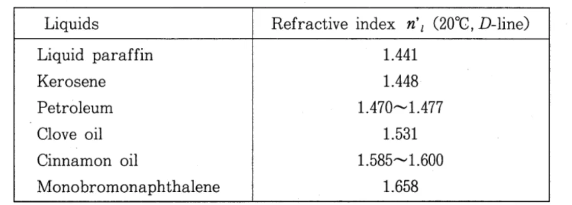
(12) 34. Memoirs of The School of B.O.S.T. of Kinki University. No. 4 (998). y A. Optical parallels. x. Film. nf Immersion layer. n~. Fig. 7. L(X, Y) = n j. •. = An'[. Liquid immersion method. g(X, Y) + {A -g(X, Y)} n~. + (nj-n~)g(X,. (31). Y) .. By omitting the fixed term A because it has no relation with phase difference, phase error of the film is eventually written as (32). Accordingly, to ms;tke the phase error due to ruggedness of the film as small as possible, it is enough to devise how to bring Inj-n'll as close as possible to zero. Refractive index nj of the film is about n = 1.554-1.557 for the film base of polyester resin system, though dependent on its emulsion. Besides, liquids in Table 1 are effective as the immersion fluid, and we can prepare a liquid with n~ equal to nj by mixing these appropriately. Employed in this examination can be the procedure in which out-of-focus image of the boundary between the film and immersion liquid is observed using a microscope (Beckman method)..

(13) 35. Table 1. Refractive indices of liquids for immersion Refractive index n'l (20°C, D-line). Liquids Liquid paraffin. 1.441. Kerosene. 1.448. Petroleum. 1.470---1.477. Clove oil. 1.531. Cinnamon oil. 1.585---1.600. Mono bromona ph thalene. 1.658. As already been evident with Eq. (20), by the way, if inserting a differential filter with amplitude transmittance proportional to x into the spatial frequency region, namely on Fraunhofer diffraction plane (x- y) amplitude distribution on the image plane obtained becomes the partial derivative of complex structure of the original object feu, v) in u direction. Similarly, insertion of "the filter proportional to y gives partial derivative of f( u, v) in v direction. If distribution of refractive index of the object is unchanged, optical path length depends on thickness of the object. In this case, intensity distribution of the image obtained with optical differentiation is in proportion to variation in the thickness. From this principle, we can obtain thickness-wise strain gradient of the object. In this chapter, we describe measurement principle for thickness-wise strain gradient of the object based on the principle in the previous section, and carry measurement of strain gradient distribution applied on a flat plate as an application. Also, we conduct experiment to confirm special effect for distribution of gradation in the human portrait, when thickness of the object is fixed, as the measurement of amplitude distribution.. 2.1 Verification of Optical Differentiation with Standard Sample First of all, measurement of phase distribution through optical differentiation is carried by means of a standard sample. When the sample is transparent and of phase structure: and we denote its distribution of thickness along W axis as g( U, V) and that of refractive index as ncC U, V), distribution of path length, namely phase, of the light wave that passes through this sample along u axis becomes as shown in Fig. 8 E,d(U, V) = ncCu, v) . g(u, v) +no . {at-g(u, v)}. (33) = noa t + {ncCu, v) -no} . g(u, v).

(14) 36. Memoirs of The School of B.O.S.T. of Kinki University No. 4 (1998). v. Fig. 8. Phase distribution of samples. where, no is refractive index of air. In this case, constant term at is independent from phase difference of the light wave that passes through the sample. Also, no = 1 usually. Eventually, when a parallel plane wave passes through this phase object, phase of the light wave yields a shift of k{n/u, v)-l} . g(u, v) from Eq.(33)lO). Thus, when the sample is a transparent substance with such features as refractive index uniformly' distributing and its amplitude transmittance being unity, amplitude distribution of the light wave that passed through this sample is given from Eq. (15) . with feu, v) = exp{jk . g(u, v)} .. (34). u. C). Fig. 9. w. Shape of standard lens.

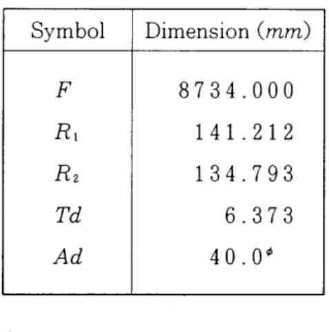
(15) 37 Table 2. Dimensions of standard lens. Symbol. Dimension (mm). F. 8734.000. Rl. 141.212. R2. 134.793. Td. 6.373. Ad. 40.0 111. Now we consider a lens as this sort of standard sample. We adopted a concave lens having a small change in its thickness and finished to accuracy of about 1.0 11m. Its external shape is shown in Fig. 9 and major dimensions in Table 2. There are following relations holding true among these: U 2+W2 =. Ri. U 2+ ( W - Td)2. =. }. R~ .. (35). Accordingly, change along u axis (same as v aXls, too, due to symmetry of rotation) becomes g(U, V). = LtW. = ~Ri-u2. (36). - {~R~-U2 +Td }. and differentiation of this Eq. (36) with respect to U glves (37) by substituting R, and R2 from Table 2, we can calculate out the value of with respect to the U value. From Eq. (34), on the other hand, amplitude distribution of the image through optical differentiation becomes {ag(U, V)/aU}. af'( U',. au'. V'). . =Jk. ag'( U',. au'. V'). exp{jkg'(U', V')}.. (38). Therefore, its intensity distribution is given from Eq. (14) as follows: . (39).

(16) 38. \lemoirs of Th e School of B.O.S.T. of Kinki University. No. 4 (998). Eventually, we can verify the value of thickness gradient of optical differentiation for the standard sample from comparison between the value geometrically obtained from Eq. (37) and the value of ~ I( U', V') obtained from Eq. (39) through optical differentiation. We describe the result of verification experiment based on the above consideration. Fig.10 shows theoretical values of thickness gradient (namely phase gradient) obtained by calculation and values from a measured curve by optical differentiation. Abscissa shows distance (Ad) from the lens center 0, while ordinate has taken the value of thickness gradient {a g'( U', V')j au'} converted with Eq. (39) from intensity distribution of the image measured with a micro photometer. By setting a reference point (we took an edge of the lens), we can put the result of measured curve upon the curve of thickness gradient obtained through calculation so as to agree with each other. With this comparison, we can measure distribution of thickness gradient with a precision of about 2.0 x 10- 4 in the optical system employed in the experiment. Accordingly, phase gradient of an object with different phase structure can be obtained in reference to Fig.10 by means of the same optical system and development processing under the same condition.. Fig.10. Differential Image of standard lens and theoretical curve. 2 . 2 Measurement of Thickness-wise Strain Gradient in In this section, study is advanced, as an application of thickness gradient aforementioned, on quantitative measurement of thickness-wise strain gradient distribution of a flat plate. For a phase object with constant refractive index and.

(17) 39. thickness distribution of g(U, V), we can obtain {og'(U', V')/oU'} with optical differentiation. Besides, g'( U', V') is thickness distribution, so its derivative is equivalent to thickness-wise strain gradient Ew' Therefore, between thickness-wise strain gradient and intensity distribution caused when a load is applied on a flat plate sample with uniform thickness, the following relation holds true:. leu', v'). ~ {~:~}2. (40). .. Then leu', v') is obtained through optical differentiation, and strain gradient can be determined from this. As the material employed, we chose polycarbonate plate ll . 12 ) that has a broad range of elasticity, uniform distribution of refraction index, and a large transmittance for wavelength of the used light source as well. Fabricated from this plate sample was a plate of 3.3 mm thick, 50 mm wide and 25 mm high, to which we applied a concentrated load PI at its center as shown in Fig.11. When taking U and V axes within the plane of this plate sample and W axis perpendicular to it, and provided as conditions of plane stress that each of stresses OW' Tuw and Tvw is zero on and within the plate, and that each of stresses au, 0v and Tuv takes averaged value of the plate m the direction of thickness, we obtain from elasticity theory as follows I3):. °v = T. uv. _ 2P1. cos. •. r. J[. = -. 2P1 J[. •. sin r. e . sin e 2. e.. (4]). cos 2 e. .. o. v. u Fig.l1. Concentrated load on semi-infinite plate.

(18) 40. ~lemoirs. of The School of B.O.S.T. of Kinki University. Therefore, if denoting elastic modulus as components of the strain as follows: tu=. -. - 2P1 v-. cos 8 (. · --. r. Ie. E. 2P. v. COS. and Poisson's ratio as. J;. we obtain. . 2 ). cos 8-v SIn 8. 8 ( SIn . 2 8-v cos 2 8 ). = - - 1- . - -. r:. 2Pl. r. V. r:. n. W. (42). cos 8. =--.-.--. E. 2. r:,. No. 4 (1998). r. .. Accordingly, partial differentiation of the above gIVes strain gradients and aEw/ av as follows:. aEw au aEw av. =. -2vP1. cos 28. =. -2vP1. sin 28. nr: nr:. r2. atw/ au. ). r2. v. v. u Fig.12. (43). u. Isostrain gradient curve in U direction. Fig.13. Isostrain gradient curve in V direction. P,. v. v. u Fig.14. Result of optical differentiation in U direction. u Fig.15. Result of optical differentiation in V direction.

(19) 41. By substituting elastic modulus Ye, Poisson's ratio v and load PI into Eq. (43) , we can obtain the distribution in which thickness-wise isostrain gradient aEw/ au and aEw/ av is constant. Figs.12 and 13 show shapes of the isostrain gradient curve in the direction of U and V, respectively. For the experiment, on the othE3r hand, >we placed the sample on the obje~t plane (P) of the optical system in Fig. 1 shown before and inserted the binary filter we developed on the diffraction plane (Q). Its differentiated image was first recorded on the image plane (S) at the filter direction TJ set at 8 = 0 (refer to Fig. 3), and then at ()= ][.The results are shown in Figs.14 and 15, respectively. Fig.14 is differential image in the U direction corresponding to Fig.12: and similarly, Fig.15 is that in the. V direction corresponding to Fig.13. The stain gradient can be quantitatively measured through photometry of the intensity distribution for these images. . Then we consider on an example that uniform compression load P2 was applied to the both sides of a rectangular plate with a circular hole as shown in Fig.16. Similarly to the previous example, we employed as the sample a polycarbonate resin plate with thickness of 3.3 mm and size of 50 x 25 mm 2, having a circular hole with diameter of 3 mm at the center. According to strength of materials, it has been known that (a())max max stays within an error of about 6 % in comparison with semi-infinite plate if the plate width is larger than 4 times (8R) the diameter of the hole (2R ). Accordingly, 25 mm width of the shortest side compared to 3 mm of the hole diameter has availed analysis with elasticity theory for semi-in finite plate. Thus thickness-wise strain component in this case is obtained as E. vP.. w. 2R2 .. = _y:2 ( 1 - -r2- cos 28) e. (44). so strain gradients in the direotions of U and V axes are gIven by the following equations: 8R 2vP2. aEw au aEw av. =. cos 38. Ye. r3. 8R 2vP2. sin 38. ). r3. Ye. (45). Drawing of isostrain gradient curve with constant aEw/aU from this gives Fig.17. in the figure ,are the sign of aEw/ au, E8 expresses convex on Symbols E8 and the sample surface while the convex, and E8 and appear alternatively. By the way, i-t is found from comparison of right sides of aEw/ au and aEw/aV that the both eventually draw the identical isostrain gradient curve with a phase difference of just ][/2. Therefore, the result for aEw/aV can be obtained simply by replacing U and V axes with each other. On the other hand, we placed the sample of Fig.16 on the object plane (P) of the optical system shown in Fig.1, and performed filtering operation on the diffraction plane (Q) by directing the filter to 8 = 0 and 8 = ][/2. Each of the differential images was recorded at the image plane (S2). The result is shown in Fig.18. This image exhibits the same pattern as isostrain distribution of Fig.17 obtained from elasticity theory.. e. e. e.

(20) 42. :vIemoirs of The School of B.O.S.T. of Kinki University. No. 4 (998). P, 2R I. l-+---------1t--,--- v. u Fig.16. Uniform load on rectangular plate with circular hole. pz. v. ~r---~--+---~ V. u Fig.17. Isostrain gradient curve around circular hole. Fig.18. U Result of differentiation of rectangular plate with circular hole. Evaluation and Conclusion There have been produced errors caused by light scattering in the vIcImty of loading point and the hole in these figures, but we observe a good agreement with the theoretical value at any portion else. If we take intensity of differential image of the standard lens as reference, it is of course possible to measure the value of {8c w / 8V}v with an accuracy within 10 - 4 over the entire field of sight I4 . 15) . In this case, however, it is needed, for matching dc levels caused by transmittance of sample or others, to take values measured at a point of the standard lens as the reference, and determine the value at other points by means of the correction curve..

(21) 43. Last, the author inserted a sample shown in Fig.19 with a fixed phase distribution, namely thickness-wise gradient, yet with some amplitude distribution, namely image with gradation, on the object plane in the optical system, and a binary filter on its diffraction plane, to obtain the result (output image) shown in Fig.20. It was found from this that differentiation in U and V directions are executed and that application of edge extraction with respect to all directions was eventually possible.. Fig.19. Example of amplitude distribution image. Fig.20 Experimental result of optical differentiation (Corresponding to e = 0 , e = J[ / 2 and all direction). This is called special effect of filtering, so to speak, in the computer graphics, in which boundary of the image is subject to differentiation followed by flat processing for portions without gradation, resulting in an effect as if image sharpening were obtained. It was verified from above experiments that the binary filter is as effective as the analogue filter so far used, and keeps time for image processing unchanged, too . Acknowledgement. The author would like to express our appreciation to Associate Professor Toshiro Matsumoto, belonging to Department of Intelligent Mechanics, Kinki University, for his kind advice and understanding in preparation for this experiment..

(22) 44. Memoirs of The School of B.O.S.T. of Kinki University. No. 4 (1998). References. ( 1) Sadahik9 Nagae, (998); Design and Development of a Binary Filter for Image Differentiation (No. 1J, Mem. SchooL B.O.S,T. Kinki University No. 3,p.45-55. ( 2) H. H. ,Hopkins, (953); On the ,Diffraction Theory' of Optical Images, Pr.oceed. Roy. Soc.2i.7 A, pA08." ' , ' (3) Kouzo Ishikuro, (1953); Optics, Ch. 1, 6, Kyoritsu Publisher, (in Japanese). ( 4) Hiroshi Kubota, (964); Ophtics, Ch. 1, Iwanami Publisher, (in Japane'se). ( 5) R.,Nagatai '~"" Iwat,a, S.:Nagae and G. Okuno, (1968); Proc. 17th Japan Na tioha:l(jong ~,Appr' .'Medi. ~p,?3-88. ( 6) B. R:"Brown 'and A. ~I. Lohman, (1966); Complex Spatial Filtering with Binary Marks, Appl. Opt. 5~' p.967." , (7) A. W. Lohm.an, D. P,. Paris and H. W. Werlich, (1967),;' 'A Computer Generated Spatical Filter, Applied to Code Translation Appl. Opt: 6, 1139. (8) A.W. Lohman and D. P. Paris, (1967); Binary Fraunhofer Holograms, ( 9) F. A. Jenkins and H. E. White, (1970); Fundamentals of Optics, Port 2, McGraw-Hill! hic. (0) Kunio Yoshihara, (966); Applied Optics, Vol. 22, 23, Kyoritsu Publisher. (1) Polycarbonate Resin Technical Material (Physical Properties), Edited by TeikokuJinken, Ltd. (1961) (12) Yuichi Kawada and three others, (1966); Material Strength Handbook, Published by the Asahi. (3) S. Timoshenko and J". N. Goodier, (951); Theory of Elasticity, Ch.4 (2 nd ed.), McGraw-Hill, Inc. (4) S. Nagae, K. Iwata and R. Nagata, (975); Measurement of Strain Distribution in Plane Metal Plate by Optical Spatial Filtering, Appl. Optics, Vol.14, No.1, p.115-123. (5) S. Nagae, K. Iwata and R. Nagata, (1975); Measurement of Surface Strain Distribution by Means of Color Display Using Optical Spatial Filtering, Appl. Optics, Vol.14, No.4, p.970-975..

(23) 45. *iJf9ttiijIJ¥~~C51 ~~~J't~Ef;]~7tm~ciJ It G 7 ~ }v>, - ~ f*Ef;]tJ:~~7Jmc: ?'j /' ~. 3. Binary e'~mj" Gt:'d)" i- 0) ~. /'~~JE L" ~fflEf;]tJ:,ttffl~,~c: L'lliJ§m~O)~~cf~ffj" GS¥-tiO). iii~fg~1g~O)7t:ftJ~iJltlJEj" Gif L ~ 'I7Jm~m~ L t:. b O)e' 35 Go i- 0)*5~" Analog filter C:. ICJ**" Digital tJ:.:f.m~c J:. G filter e' b .5!fftJ:*5~iJ~f~ G tL G L. C: iJ~lit~:g ~ tL t:o. -1.7". f1Lm ~cMlj" G7t:ftJ ti-JEe' 35 GiJ~". 1JN~~~c Mlj"·G 7t:ftJ ti~ra'Ef;] ~c~{t L L ~ 'I GiOOf~. O)J't~Ef;]~7tm b ICJIr.f~c~~ t:iJ~" L. O)t~~~c iOOftiJ~f~. O)t~~ C: ICJ**". if L ~ 'I t:tl:t.J. GtL G L. C: iJ~lit~:g ~ tL t:o. ErfO) C: ~ 'I. b Analog filter. L.~" t:tl:t.JiOOf~O)~cijdc*5fflJtiVt*d)~~mf~~c J:.. G t: 'd)" r - >' }vEf;] tJ:~IJI!B~ra' timtE O)?' ~ >' }v •. ~'IftL~'d)LrEJ7tM¥ff~~. ~ tLtLt~'". I) 7. }v >' -1. tJ: ~ 'I C: Ji!lb tL G0. ::J /'. 1::0 .:L. G7 -. TO -7 Ef;]tJ:~mHcWl"?. >' ~c ti@ iJ~ ~c:& t~r tJ: ~ 'I iJ~". b--:J CCD tJ j :7 tJ: C'e'~L~?'~ >' }v~IJI!e'~ G ?'/'{ -1. 1.. e'. * /' :7 -1 /'. L. A iJ~~~. ~IJI!iJ~PJff~tJ:J't~Ef;]il&W Y A T 1.. O)~m b ~PJff~e' ti.

(24)