サプライチェインネットワークにおけるロバストな均衡モデルについて (最適化技法の最先端と今後の展開)

全文

(1)109. 数理解析研究所講究録第2027巻 2017年 109-124. サプライチェインネットワークにおける. ロバストな均衡モデルについて横浜国立大学国際社会科学府平野達也 Sciences, Yokohama National University. Graduate School of International Social. 横浜国立大学国際社会科学研究院成島康史 Faculty of International Social Sciences, Yokohama National University. Introduction. 1. Supply chains are connections of process including procurement of raw materials, production, ship‐ ping and selling for a product. Supply chain management is one of main objects in management science, and hence many researchers have proposed mathematical models to optimize or analyze supply chain networks. In this paper, we focus on competitive supply chain networks. Because supply chains involve many decision‐makers (called players) and they independently decide their behaviors, competitive situations often occur. To analyze, Nagurney et al. [10] proposed a supply chain network equilibrium (SCNE) model which is constructed by the manufacturers, the retailers and the demand markets. Yamada et al. [18] extended the SCNE model by considering the behav‐ iors of the distribution centers. Hammond and Beullens [5] developed a model for closed‐loop supply chain with the manufacturers and the consumer markets considering returns of the products and evaluated the effect of a legislation. Yang et al. [19] extended this closed‐loop model to a general closed‐loop supply chain network with the raw material suppliers, the manufacturers, the retailers, the recovery centers and the demand markets. Li and Nagurney [8] treated a quality competition with the suppliers, the producing firms and the demand markets and evaluated the quality of the products. Nagurney [9] considered a freight service provision network model with the disaster relief organizations, the freight service providers and the demand points. Nagurney et al. [11] dealt with a network model for post‐disaster humanitarian relief by NGOs which is constructed by NGOs, victims and donors.. Recently, particular many vulnerabilities. as. attention is to natural. paid to the risk management of supply chains. Supply chain has disasters, business fluctuations, demand and cost uncertainties. [17] suggested. that supply chains face the many kinds of risk factor and supply chains were disrupted, so it is necessary to deal with these risks. Kleindorfer and Saad [7] pointed out the necessities of three tasks which are Specifying sources of risk and vulnerabilities, Assessment, and Mitigation (SAM). Tang [16] defined supply chain risk management (SCRM) as the management of supply chain risks through coordination or collaboration among the supply chain partners so as to ensure profitability and continuity. Also, there are many researches analyzing the optimal behavior as to risks by using a mathematical model. Dong et al. [4] expanded the SCNE model in [10] to a equilibrium model with a demand. and. so on.. there. are. Wu et al.. many. cases. that.

(2) 110. uncertainty. Bertsimas and Thiele [3] analyzed inventory management problems under the demand and cost uncertainties. Qiang et al. [13] developed a supply chain network model with uncertainty in costs and demand. In addition, they proposed a supply chain network performance measure. Pishvaee et al. [12] dealt with a market to market closed‐loop supply chain network. In their research, demands, returns and transportation costs are assumed as uncertain factors. Baghalian et al. [1] developed a multi‐supply chain network model considering demand uncertainties and disruption risks. These researches analyzed a supply chain network with uncertainties in demand or cost. But they did not consider a model which has uncertainties in the other players strategies. In actually, there are many cases which players in the supply chain can not know the others strategies exactly. The aim of this paper is to consider the case that there are uncertainties in competitors strategies in the SCNE model in. [10].. In this paper,. we assume. that. some. firms. can. not know the exact value. of. competitors strategies. We also assume that under these uncertainties, they minimize their cost for the worst case. This approach is called robust optimization or robust methodology. According to Bertsimas and Thiele [3], the robust methodology can be understood as a reasonable worst‐case approach. So we call the model considered in this paper robust SCNE model. 2. Robust SCNE model. In this. develop a robust supply chain network equilibrium model. The network that we Figure 1. In this model, there are m manufacturers, n retailers (or wholesalers) and 0 demand markets. The manufacturers produce products and delivery them to the retailers. The retailers buy the products from the manufacturers and sale them to the demand markets. The demand markets buy the products from the retailers. Each manufacturer minimizes his total cost by deciding the amount of the products shipped to the retailers. Each retailer minimizes his total cost by deciding the amount of the products ordered to each manufacturer and the products sold to each demand market. Each demand market decides the purchase volume and the market price which satisfies the equilibrium conditions described later. We assume that each manufacturer and retailer cannot know exactly strategies of the other manufacturers and retailers respectively. We also assume that they minimize their cost for the worst case. We formulate their problems as second‐order cone programming problems and also reformulate them as a VIP. section,. we. consider is shown in. Figure First,. we. 1:. Supply. chain network. define the variables for this model. For. q_{ij}(\geq 0) w_{jk}(\geq 0) p_{k}(\geq 0). :. the amount of the. :. the amount of the. :. the market. price. equilibrium model.. i=1,. \cdots. ,. m,. j=1,. \cdots,. n,. k=1,. \cdots, 0 :. products shipped by manufacturer i to retailer j, products sold by retailer j to demand market k,. at demand market k..

(3) 111. As for these. variables,. define. we. some. vectors. as. follows:. q_{i}. := (q_{i1}, \cdots, q_{in})^{T}, q_{j} := (q_{1j}, \cdots, q_{mj})^{T}. w_{j}. := (w_{j1}, \cdots, w_{jo})^{T\prime},. w.k := (w_{1k}, \cdots, w_{nk})^{T},. q_{-i}. := (q_{1}^{T}, \cdots, q_{i-1}^{T}., q_{i+1}^{T}., \cdots, q_{m}^{T}.)^{T},. q-j := (q_{1}^{T}, \cdots, q_{\dot{}-1}^{T}, q_{j+1}^{T}, \cdots, q_{n}^{T})^{T}, w_{-\mathrm{j} . := (w_{1}^{T}, \cdots, w_{j-1}^{T}., w_{j+1}^{T}., \cdots, w_{n}^{T}.)^{T}. w_{-k} := (w_{1}^{T}, \cdots, w_{k-1}^{T}, w_{k+1}^{T}, \cdots, w_{o})^{T}, p := (p_{1}, \cdots,p_{0})^{T}. Note that q_{i} is a variable of manufacturer i, q_{j} and w_{j} are variables of retailer j , and w_{k} and p_{k} are variables of demand market k As for the price of each product, we define as follows: .. .. .. We also. use. $\rho$_{ij}. :. $\pi$_{j}. :. the price of the the price of the. following. the. product charged by retailer j to manufacturer i, product charged by demand market k to retailer j.. notations:. $\rho$_{i}. := ($\rho$_{i1}, \cdots, $\rho$_{in})^{T}, $\rho$_{j} := ($\rho$_{1j}, \cdots, $\rho$_{mj})^{T} The. 2.1. problems solved by the manufacturers. We consider the. ufacturer. We. problem solved by the manufacturers. We define the following functions. f_{i}(q_{i}., q_{-i}.). :. a. production. c_{ij}(q_{ij}). :. a. transaction cost between manufacturer i and retailer. assume. that \mathrm{c}_{ij} is. manufacturer i. convex.. (namely,. q_{i}. ). manufacturers procure the the. raw. for. man‐. i(i=1, \cdots, m) :. materials may. product function depends. on. i,. only. not. j(j=1, \cdots, n). .. the decision variable of. (namely, q_{-i}. ), that is, if the products from a same supplier, a competition for affect the production cost. In this paper, we define f_{i}(q_{i}., q_{-i}.) as. but also that of the other manufacturers. raw. occur. A. cost function of manufacturer. materials of the. and. follows:. f_{i}(q_{i}., q_{-i}.) :=(\displaystyle \sum_{j=1}^{n}q_{ij})(a_{i }+b_{i1}\sum_{j=1}^{n}q_{1j}+\cdots+b_{i }\sum_{j=1}^{n}q_{ij}+\cdots+b_{im}\sum_{j=1}^{n}q_{mj}) where a_{ii} and b_{is} (s=1, \cdots , m) dimensions whose all components are. b_{is}. .. are. are. ,. nonnegative scalars. Let a_{i} denote a column vector in n B_{is}\in \mathbb{R}^{n\times n} denote a matrix whose all components. a_{ii} and. Then it follows that. f_{i(q_{i}.,q_{-i}.)=a_{i}^{$\tau$_{q_{i}.+q_{i}^{$\tau$_{B_{i} q_{i}.+\sum_{l\neq\dot{\circ} ^{m}q_{i}^{T}B_{ilq_{l} }.l=1^{\cdot}. .. ..

(4) 112.

(5) 113. where. (q_{1}^{T},. T:=\{(q^{T}, s^{T})^{T}|0\leq q, \Vert M_{it}B_{il}q_{i}.\Vert\leq s_{il}(l=1, \cdots, i-1, i+1, \cdots, m, i=1, \cdots, m)\},. \cdots. ,. q:=. q_{m}^{T}.)^{T} and :=(s_{1}^{T}, \cdots, s_{m}^{T})^{T} s. 2.2. The. Next,. we. problems solved by. consider the. the retailers. problem solved by the retailers. We define the following function for retailer. j(j=1, \cdots, n) : hj (q.j, q_{-j}) According. to. Nagurney product. associated with. et al.. [10],. :. the. a. handling. handling. . In this paper,. we. cost of retailer. cost may include. define. h_{j}(q_{\dot{}}, q_{-j}). as. . j. the. display. and storage cost. below:. h_{j}(q_{j}, q_{-j}):=(\displaystyle \sum_{i=1}^{rn}q_{ij})($\delta$_{i }+$\gamma$_{j1}\sum_{i=1}^{m}q_{i1}+\cdots+$\gamma$_{j }\sum_{i=1}^{m}q_{ij}+\cdots+$\gamma$_{jn}\sum_{i=1}^{m}q_{in}) $\delta$_{j } and $\gamma$_{jt} (t=1, \cdots , n) dimensions whose all components where. are. $\gamma$_{jt}. .. Then, the function (2.4). are are. nonnegative scalars.. $\delta$_{j }. and. is rewritten. Let. $\delta$_{j}. denote. $\Gamma$_{jt}\in \mathbb{R}^{m\times m}. denote a. ,. (2.4). column vector in. a. matrix whose all. m. components. as. h_{j}(q.j,q_{-j})=$\delta$_{j}^{T}q_{j}+q_{j}^{T}$\Gam a$_{j}q_{j}+\displaystyle\sum_{r=1,r\neq\mathrm{j}^{n}q_{j}^{T}$\Gam a$_{jr}q_{r}. Note that the total sales for the is. $\rho$_{j}^{T}q_{\dot{}. We. products of. $\pi$_{j}\displaystyle \sum_{k=1}^{o}w_{jk}. retailer j is. that the retailers must not. assume. cause. an. and the total. stocking cost goods. That is, for. absence of the. retailer j , the total stock of the products (=\displaystyle \sum_{i=1}^{m}q_{ij}) must not be less than the total sales amounts (=\displaystyle \sum_{k=1}^{o}w_{jk}) If we denote the total cost of retailer j by $\Phi$_{j}(q_{j}, q_{-j} , wj the total cost of him is .. given by. $\Phi$_{j}(q_{j},q-j,w_{j}.)=-$\pi$_{j}\displaystyle\sum^{o}w_{jk}+$\rho$_{j}^{T}q_{j}+$\delta$_{j}^{T}q_{j}+q_{j}^{T}$\Gam a$_{j}q_{j}+\sum_{r\neqj}^{n}q_{j}^{T}$\Gam a$_{jr}q_{r}k=1^{\cdot}\cdot\cdot.\cdotr=1^{\cdot}\cdot\cdot We. assume. that retailer j cannot know the exact value of q.-j but estimates q_{r} as \tilde{q}_{r} :=q_{r}+ defimte matrix , where N_{jr}\in \mathbb{R}^{m\times m} is a symmetric positive. N_{jr} $\Delta$ v_{r} (r=1, \cdots , j-1, j+1, \cdots, n). and $\Delta$ v_{r}\in \mathbb{R}^{m} satisfies \Vert $\Delta$ v_{r}\Vert\leq 1 We also assume that he minimizes his cost for the worst case by using the robust approach same as the problems solved by the manufacturers. Then, retailer j s .. cost function for the worst. case. \tilde{ $\Phi$}_{i}(q_{j}, q_{-j}. ,. wj. ) is. \displaystyle \tilde{ $\Phi$}_{j}(q.j, q_{-j}, w_{j}.)=\max\{$\Phi$_{i} ( q j \tilde{q}_{-j}, w_{j} .. where. \tilde{q}.-j. :=. ( \tilde{q}_{1})^{T},. \cdots. ,. ,. (\tilde{q}_{j-1})^{T}, (\tilde{q}_{j+1})^{T}, \cdots, (\tilde{q}_{n})^{T})^{T},. q_{r}+N_{jr} $\Delta$ v_{r}|\Vert\triangle v_{r}\Vert\leq 1\} Here, V_{-j} .. is the. uncertainty. \tilde{q}.-j\in V_{-j}\},. V_{-j}:=\displaystyle \prod_{r\neq j}^{n}r=1V_{\dot {}r}. set for retailer. .. j. .. and. V_{jr} :=\{\tilde{q}_{r}=. So the function which. retailer j should minimize is. \displaystyle \tilde{ $\Phi$}_{i}(q_{j}, q_{-j}, w_{j}.)=-$\pi$_{j}\sum_{k=1}^{o}w_{jk}+$\rho$_{j}^{T}q_{j}+$\delta$_{j}^{T}q_{j}. +q_{j}^{T}$\Gamma$_{j }q_{j}+\displaystyle \sum_{r\neq jr\neq \mathrm{j} ^{n $\tau$.n}r=1q_{j}$\Gamma$_{jr}q_{r}+\sum r=1\Vert\triangle\max_{v_{r}|\leq 1}q_{j}^{T}$\Gamma$_{jr}N_{jr} $\Delta$ v_{r}..

(6) 114. \displaystyle \Vert\triangle\max_{v_{r}|\leq 1}q_{j}^{T}$\Gamma$_{jr}N_{jr}\triangle v_{r}=\Vert N_{jr}^{T}$\Gamma$_{jr}^{T}q_{j}\Vert=\Vert N_{jr}$\Gamma$_{jr}q_{j}\Vert. Note that. second‐order. following. cone. .. Accordingly,. retailer. j. solves the. programming problem:. \displaystyle \min_{q_{j},w_{j}.,t_{j} \hat{ $\Phi$}_{j}(q_{j}, q-j, w_{j}., t_{j})=-$\pi$_{j}\sum_{k=1}^{o}w_{jk}+$\rho$_{j}^{T}q_{j}+$\delta$_{j}^{T}q_{j}+q_{j}^{T}$\Gamma$_{j }q_{j} +\displaystyle \sum_{r=1}^{n}q_{j}^{T}$\Gamma$_{jr}q_{r}+\sum_{r=1}^{n}t_{jr}r\neq j.\cdot f\neq j. 0\leq q_{j}, 0\leq w_{j}., \displaystyle \sum_{k=1}^{o}w_{jk}\leq\sum_{i=1}^{m}q_{ij}, \Vert N_{jr}$\Gamma$_{jr}q_{j}\Vert\leq t_{jr} (r=1, \cdots,j-1,j+1, \cdots, n). \mathrm{s} .t.. where. t_{j}. :=. given by. (t_{j1}, \cdots , t_{jj-1}, t_{jj+1}, \cdots, t_{jn})^{T}. .. Let. S_{j}. denote the feasible set of. (2.5),. (2.5) ,. and then. S_{j}. is. S_{j}:=\displaystyle \{(q_{j}^{T}, w_{j}^{T}, t_{j}^{T})^{T}|0\leq q_{j}, 0\leq w_{j}., \sum_{k=1}^{o}w_{jk}\leq\sum_{i=1}^{m}q_{ij}, \Vert N_{jr}$\Gamma$_{jr}q_{j}\Vert\leq t_{jr} (r=1, \cdots,j-1,j+1, \cdots, n)\}.. convex set and the objective function \hat{$\Phi$}_{j} is convex with q_{j}, w_{j} and t_{j}, programming problem. By using a Lagrange multiplier $\xi$_{j}\in \mathbb{R}+ for given q.-j, the optimal condition for (2.5) is given by the following (see [2], for example) :. Because. (2.5). is. S_{j}. is. a. nonempty. .. a convex. ,. ++(\d\ispdilaysstplela\sysumt_y{kl=e1}^\s{o}\u{($m_\xi${_i{j=}^1}*\sûm{m_{i=}1q}^_{m{i}\j}{(^$\{r*h}o-$\_s{iju}^{m_*+-\f{rkac=1}{\partî{loh_}{wj}(q_^{{*}jqk.)}{^$\{p*}i$)_({j$}^\xi*)^{\$pa_rt{ijl}q-$_{i\xi\mat$hrm_{{jj}}(^w{_*{}jk)}-$\xi$_{j}^*(q_{ij}-q_{ij}^{*)\}-w_{jk}^{*\ }. (2.6). +\displaystyle \sum_{r\neq \mathrm{j} ^{n}r=1(t_{jr}-t_{jr}^{*})\geq 0, \foral (q_{j}^{T}, w_{j}^{T}, $\xi$_{j}, t_{j}^{T})^{T}\in\hat{S}_{j}, where. \hat{S}_{j}:=\{(q_{j}^{T}, w_{j}^{T}, $\xi$_{\dot{} , t_{j}^{T})^{T}|0\leq q_{\mathrm{j} , 0\leq w_{j}., 0\leq$\xi$_{j}, \Vert N_{jr}$\Gamma$_{jr}q_{\mathrm{j} \Vert\leq t_{jr} (r=1, \cdots,j-1,j+1, \cdots, n)\}. Also, by gathering (2.6). as. for all. retailers,. we. get the following equilibrium condition:. ++\di\displasysptllea\yssumt_y{j=le1}^{\sn\suumm__{k={1j}=^{o1}\{(^$\{xni$}_({j\}^s*-uwm__{jk}^{{*i\=1}}\sûm{m_{j=}1q}^{_n{\isju}m^_{{i*=}1-}\^{ms}u\{m_($\rh{ok$_=1}{ij}^*^+\{forac}{w\p_ar{tijklh}_^{j}{(q*}_){\(m$at\xihrm{j$}^_*{,qj_}{--}$^*\xi\cdo$t)}_{${\jp}i^$_{{j*}}^)*){q_ij}(w_{jk}-$\xi$_{j}^*(q_{ij}-q_{ij}^*)\}. (2.7). +\displaystyle \sum_{j=1}^{n}\sum_{r\neq j}^{n}r=1(t_{jr}-t_{jr}^{*})\geq 0,. \forall(q^{T}, w^{T}, $\xi$^{T},t^{T})^{T}\in\hat{S}, where. j=1,. \cdots. :=\{(q^{T}, w^{T}, $\xi$^{T}, t^{T})^{T}|0\leq q, 0\leq w, 0\leq $\xi$, \Vert N_{jr}$\Gamma$_{jr}q_{j}\Vert\leq t_{jr}(r=1, n)\}, :=(w_{1}^{T}, \cdots, w_{n}^{T}.)^{T}, $\xi$ :=($\xi$_{1}, \cdots, $\xi$_{n})^{T} and t:=(t_{1}^{T}, \cdots, t_{n}^{T})^{T} ,. w. \cdots. ,. j-1,j+1,. \cdots. ,. n,.

(7) 115. 2.3. The conditions for the demand markets. Finally,. we. consider conditions which should be satisfied in the demand markets. For. define the. we. d_{k}(p). :. a. demand function of demand market. g_{jk}(w_{k}, w_{-k}). :. a. transaction cost between demand market k and retailer. We. assume. that. k=1,. \cdots,. 0,. functions:. following. the. on. equilibrium,. the. following. k,. conditions. are. j(j=1, \cdots , n). .. satisfied for demand market. k(k=1, \cdots, 0) :. \left\{ begin{ar ay}{l $\pi$_{j}+g_{jk}(w.k,w_{-k})=p_{k}\mathrm{i}\mathrm{f}w_{jk}>0,\ $\pi$_{j}+g_{jk}(w_{k},w_{-k})\geqp_{k}\mathrm{i}\mathrm{f}w_{jk}=0, \end{ar ay}\right.. (2.8). \left\{ begin{ar y}{l d_{k}(p)=\sum_{j=1}^{n}w_{jk}\mathrm{i}\mathrm{f}p_{k}>0,\ d_{k}(p)\leq\sum_{j=1}^{n}w_{jk}\mathrm{i}\mathrm{f}p_{k}=0. \end{ar y}\right.. (2.9). a demand market purchases the products from retailer j sum of price of the product equals to the market price and when the demand market does not buy any products, sum of the transaction cost and the price of the product surpasses the market price. Condition (2.9) means that, when the market price is positive, the market demand equals to the purchase volume of the products from the retailers and when the market price is 0, the market demand belows the purchase volume of the products from the retailers. For given w_{-k} and p_{-k} the conditions (2.8) and (2.9) can be rewritten as follows:. Condition. (2.8). means. that,. when. ,. the transaction cost and the. ,. \displaystyle \sum_{j=1}^{n}\{($\pi$_{j}^{*}+g_{jk}(w_{k}^{*}, w_{-k})-p_{k}^{*})(w_{jk}-w_{jk}^{*})\} +(\displaystyle \sum_{j=1}^{n}w_{jk}^{*}-d_{k}(p_{k}^{*},p_{-k}) (p_{k}-p_{k}^{*})\geq 0. (2.10). ,. \forall w_{k}\in \mathbb{R}_{+}^{n}, p_{k}\in \mathbb{R}_{+}. By gathering (2.10) for. all demand. markets,. we. obtain. \displaystyle \sum_{k=1}^{o}\sum_{j=1}^{n}\{($\pi$_{j}^{*}+g_{jk}(w_{k}^{*}, w_{-k}^{*})-p_{k}^{*})(W_{jk-w_{jk}^{*})\} +\displaystyle \sum_{k=1}^{o}\{(\sum_{j=1}^{n}w_{jk}^{*}-d_{k}(p_{k}^{*},p_{-k}^{*}) (p_{k}-p_{k}^{*})\}\geq 0 ,. \foral w\in \mathbb{R}_{+}^{no}, p\in \mathbb{R}_{+}^{k}. 2.4. Reformulation. By gathering (2.3), (2.7). as a. VIP. and. (2.11),. we. get. \displaystyle \sum_{i=1}^{m}\sum_{j=1}^{n}\{(\frac{\partial f_{i}(q_{i}^{*}.,\mathrm{q}_{-i}^{*}.)}{\partial q_{ij} ++(q_{ij}-q_{i.i}^{*})\}. +\displayst le\sum_{j=1}^{n}^{+\sum_{j=1}^{n}(\sum_{i=1}^{m}^{\sum_{k=1}^{o}q_{ij^*}-\sum_{k=1}^{o}^{\(g_{jk}w_{jk^{*})($\xi$_{j}-$\xi$_{j}^*)(w_{k}^{*,w_{-k}^{*)-p_{k}^{*+$\xi$_{j}^*)\backsla h^{w_{jk}-w_{jk}^{*)\} +\displaystyle \sum_{k=1}^{o} (\sum_{j=1}^{n}w_{jk}^{*}-d_{k}(p_{k}^{*},p_{-k}^{*}) (p_{k}-p_{k}^{*})\}. +\displaystyle \sum_{i=1}^{m} \sum_{ $\iota$\neq i}^{m}l=1(s_{il}-s_{il}^{*})\} +\displaystyle \sum_{j=1}^{n} \sum_{r\neq j}^{n}r=1(t_{jr}-t_{jr}^{*})\}\geq 0,. \forall(q^{T}, w^{T}, $\xi$^{T}, p^{T}, s^{T}, t^{T})^{T}\in K,. (2.11).

(8) 116. where. K:=\{(q^{T}, w^{T}, $\xi$^{T},p^{T}, s^{T}, t^{T})^{T}|0\leq q, 0\leq w, 0\leq $\xi$, 0\leq p, \Vert M_{il}B_{il}q_{i}.\Vert\leq s_{il} (l\neq i, i=1, \cdots , m) , \Vert N_{jr}$\Gamma$_{jr}q_{j}\Vert\leq t_{jr}(r\neq j, j=1, \cdots , n Therefore the all. players problems. are. reformulated. Find x^{*}\in K such that. as. the VIP:. F(x^{*})^{T}(x-x^{*})\geq 0,. \forall x\in K. ,. (2.12). where. x:=\left(bgin{ary}l q\ w $\xi p\ s t\end{ary}\ight). and. F(x):=\ovalb{tsmREJCT -$\xi_{1}dsplaytefrc(q.o,)nmhz+\d1}a{prtil_q-$xgn(w,)o^fcm:+h\}{1i_partlq-0d$xng(wO,)cosum^j=:+.}{\frath_1qpil$n()w-cdosumk=^{},\argft_qpil1.h(-)mwk^+c{n}$\xdo,:ts valbmREJCT}..

(9) 117. 3. Numerical. Now. (2.12). It is difficult to solve VIP (2.12) directly problem has non‐differentiaule functions in set K In the paper, we reformulate (2.12) second‐order cone complementarity problem. Note that K can be written as follows: we. experiments. introduce the solution method of VIP. because this as a. .. K:=\{(q^{T}, w^{T}, $\xi$^{T},p^{T}, s^{T}, t^{T})^{T}|(q^{T},w^{T},$\xi$^{T},p^{T})^{T}\in \mathbb{R}_{+}^{ $\sigma$},. (s_{il}, q_{i}^{T}B_{il}M_{il})^{T}\in \mathcal{K}^{1+n}(t=1, \cdots, i-1, i+1, \cdots, m, i=1, \cdots, m). ,. (t_{\dot {}r}, q_{j}^{T}$\Gamma$_{jr}N_{jr})^{T}\in \mathcal{K}^{1+m}(r=1, \cdots,j-1,j+1, \cdots, n, j=1, \cdots, n)\}, where cone. $\sigma$. :=mn+no+n+0 , and. \mathcal{K}^{1+n} and \mathcal{K}^{1+m}. are. 1+n and 1+m dimensional second‐order. dimensional second‐order. respectively. Generally, the 1+ $\zeta$. cone. \mathcal{K}^{1+ $\zeta$}. is defined. by. \mathcal{K}^{1+ $\zeta$}:=\{y=(y_{1}, y_{2}^{T})^{T}|y_{1}\geq\Vert y_{2}\Vert, y_{1}\in \mathbb{R}, y_{2}\in \mathbb{R}^{ $\zeta$}\}. We define \mathcal{K}^{1}. by \mathbb{R}+\cdot. We define \mathcal{K} and. $\theta$(x). as. \displaytemhc{K}:=\abR_+^$sigm}\teprod_{=1^m l,\neqi}{mathcK^+1\iesprod_{j=}^n 1,r\eqj{}mathclK^+1,$\e(x):=lft{bginary} q\w$xip\ s_{12}MBq_{1\ sm-}M_{1Bm-}q\ t_{12N}$Gam_{\thrl}2q1 _{n-\N1}$Gam_{n-q \edary}ight.. (2.12) is rewritten by K=\{x| $\theta$(x)\in \mathcal{K}\} Therefore, from KKT (2.12) can be reformulated as the following mixed second‐order cone complementarity problem (see [14] and [15]): Then, the. set K. conditions of VIP. appearing. (2.12),. in. .. VIP. Find. such that. (x, $\lambda$)\in \mathbb{R}^{ $\nu$}\times \mathbb{R}^{ $\tau$} F(x)-\nabla $\theta$(x) $\lambda$=0. (3.1). ,. $\theta$(x)\in \mathcal{K}, $\lambda$\in \mathcal{K}, $\theta$(x)^{T} $\lambda$=0,. where. \mathrm{v}. := $\sigma$+m(m-1)+n(n-1) and $\tau$ := $\sigma$+m(m-1)(n+1)+n(n-1)(m+1) (3.1) by ReSNA [6] to analyze the impact of uncertainties on the shipments, .. the. prices, Nagurney et al. [10] for each cost function and demand function. The number of the manufacturers, the retailers and the demand markets are two respectively. In these numerical experiments, we consider the following two cases with a constant $\alpha$ : We solve. the. profits. and the total. supply chain. cost per unit. We choose the. parameters. same as.

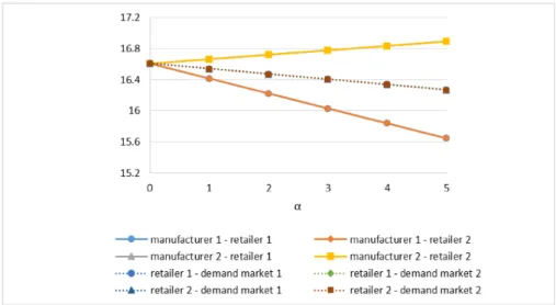
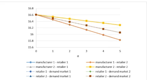
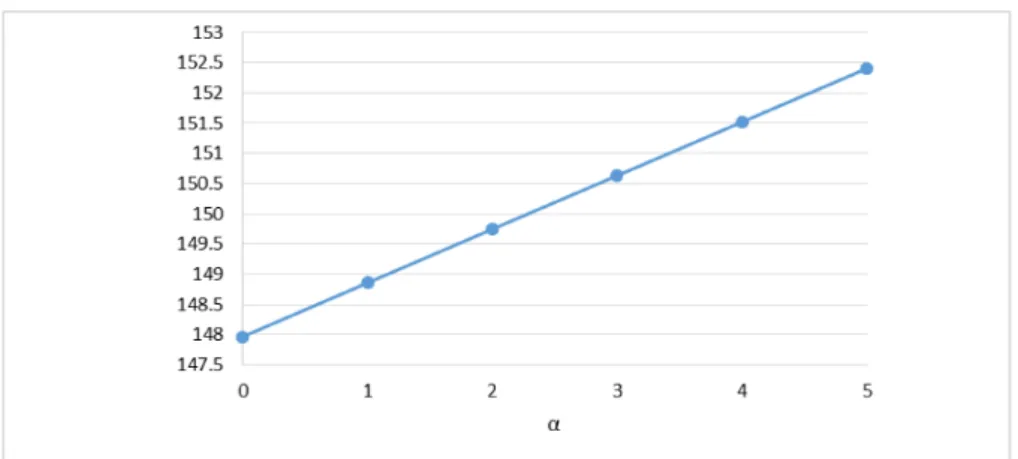
(10) 118. Case 1.. Manufacturer 1 does not know the exact behavior of manufacturer 2 and the parameters. for the uncertainties. given by. are. M_{12}=$\alpha$\times\left(\begin{ar ay}{l} 1&0\ 0&2 \end{ar ay}\right),M_{21}=\left(\begin{ar ay}{l} 0&0\ 0&0 \end{ar ay}\right). Case 2.. Neither manufacturer 1. nor. manufacturer 2 knows the exact value of the opponent each. other and the parameters for the uncertainties. are. given by. M_{12}=$\alpha$\times\left(\begin{ar ay}{l} 1&0\ 0&2 \end{ar ay}\right),M_{21}=$\alpha$\times\left(\begin{ar ay}{l} 1&0\ 0&1 \end{ar ay}\right). For both the cases,. we. exact behavior of the. both the cases, there. change. $\alpha$. from 0 to 5. When. opponent. The larger are. $\alpha$. $\alpha$. equals. to 0 , each. manufacturer knows the. gets, the larger the uncertainties get. too.. Also for. not uncertainties between the retailers.. The results of the experiments are shown in Figures 2‐9. In Figure 2 and Figure 6, [circles line] and [diamonds and solid line], and [triangles and solid line] and [squares and solid. and solid. line]. overlapping respectively. The rest four dashed lines are overlapping too. In Figure 3 and the line of [circles and solid line] and [diamonds and solid line], [triangles and solid line] 7, Figure are. [squares and solid line], [circles and dashed line] and [diamonds and dashed line], and [triangles line] and [squares and dashed line] are overlapping respectively. In Figure 4 and Figure 8, [triangles and solid line] and [squares and solid lines] are overlapping. and. and dashed. Seeing Figure 2, the larger the uncertainty gets, the fewer the amount of the products shipped by manufacturer 1 gets. But the amount of the products shipped by manufacturer 2 is increasing. Sum of the amount of the products shipped by retailer 1 and 2 get fewer. In Figure 3, the prices charged by the demand markets to the retailers are getting higher. We see that the profit of manufacturer 1 is decreasing while the profit of manufacturer 2 is decreasing from Figure 4, and the total cost per unit is getting higher from Figure 5. Seeing Figure 6, if both the manufacturers have the uncertainties, they decrease the amounts of the products. But manufacturer 1, who has more uncertainty than manufacturer 2, produces fewer. We see that the price charged by the retailers to manufacturer 2 is getting lower from Figure 6, and the profit of manufacturer 2 is decreasing from Figure 8. Comparing Figure 5 and Figure 9, the total supply chain cost per unit for the case 2 is higher than case 1. In both the cases, the larger the uncertainties get, the more retailers get profit..

(11) 119. 2 $\alpha$\}. ... 0. 1. 2. 4. 3. 5. $\alpha$. \cdots. the market price set by demand market 1. Figure. 3: The effects of uncertainties. \blacksquare\cdots the market on. the prices. $\mu$ \mathrm{i}\mathrm{o}\mathrm{e}. set \mathrm{b}. (case 1).. 何mand matket2.

(12) 120. 0 1 2 $\alpha$ 3 4 \mathrm{s} 1 \rightarrow manubdurer 1. -\mathrm{m}\mathrm{a}\mathrm{n}\mathrm{u}\mathrm{f}\mathrm{a}\mathrm{c}\mathrm{t} $\iota \kappa$ \mathrm{e}\mathrm{r}2. retailer 1. -\mathrm{}.\mathrm{e}\mathrm{t}\mathrm{a}.\mathrm{i}.|\mathrm{e}r2\wedg\cdot\cdot\sim-\cdot\cdot-\cdot-\cdot\backslah\cdot\backslah\cdots\cdot\ve\cdot-. —. Figure. 147.. 4: The effects of uncertainties. on. the. profits (case 1).. 5012345\underline{|} $\alpha$. \cdots--\cdot\cdot-. Figure. 5: The effects of uncertainties. on. the total. supply chain. costs. (case 1)..

(13) 121. 0. 1. 2. 4. 3. 5. $\alpha$. — manufacturer 1‐retailer 2. \rightarrow manufacturer 1‐retailer 1 — \cdots. manufadurer 2‐retai | er 1. 6: The effects of uncertainties. 0. 1. er. 2. *\cdots retailer 1- demand \mathrm{m}\mathrm{a}*\mathrm{e}\mathrm{t}2. \mathrm{b}\cdots retailer 2‐ demand market 1. Figure. manufacturer 2‐retai. ‐ltl. retailer 1‐demand market 1. \cdots. on. 2. the. 3. retailer 2-\mathrm{d}\mathrm{e}\mathrm{m}\mathrm{a}\mathfrak{n}\mathrm{d}. \mathfrak{m} atket2. shipments (case 2).. 4. 5. — manufadurer 1‐ retailer 2 --. \cdots. manufadurer 2-\mathrm{r}\mathrm{e}\mathrm{t}\mathrm{a}\mathrm{i}\mathrm{l}\mathrm{e} $\tau$ 2 retailer 2‐ demand market. \blacksquare\cdots the market. Figure 7: The effects of. uncertainties. on. the prices. price. set. Uy demand market. (case 2).. 2.

(14) 122. 0. 1. 2. 3. 4. 5. $\alpha$. Figure. 147.. \rightarrow—manufacturef1. \rightarrow- manufadurer 2. — retailer 1. — retailer 2. 8: The effects of uncertainties. on. the. profits (case 2).. \mathrm{S}\mathrm{L}_{-} 0. 1. 3. 2. \mathrm{s}. 4. $\alpha$. Figure. 9: The effects of uncertamties. on. the total. supply chain. costs. (case 2)..

(15) 123. Conclusions. 4. In the paper, we have developed a robust SCNE model which value of other players strategies. In addition, we have given. some some. players. cannot know the exact. numerical experiments. For a variables and demands such as. future research, to consider the model with uncertainties in players [4] simultaneously is an interesting topic. Also numerical experiments with realistic parameters is an. important issue.. Acknowledgements by the Grant‐in‐Aid for Young Scientists (B). The second author is. supported. Japan Society for the. Promotion of Science.. in part. 25870239 of. References. [1]. Baghalian, S. Rezapour and R.Z. Farahani, Robust supply chain network design with ser‐ against disruptions and demand uncertainties: A real‐life case. European Journal of Operational Research, 227 (2013), 199‐215.. A.. vice level. [2]. Tsitsiklis, Parallel and Distributed Computation: Numerical Methods. Prentice‐Hall, Englewood Cliffs, NJ 1989.. D.P. Bertsekas and J.N.. ,. Thiele, A robust optimization approach to supply chain management. Integer programming and combinatorial optimization, Springer‐Verlag Berlin Heidelberg (2004), S6‐100.. [3]. D. Bertsimas and A.. [4]. J.. In: D. Bienstock and G. Nemhauser eds.. Dong,. demands.. Zhang and A. Nagurney, A supply chain network equilibrium model with random European Journal of Operational Research, 156 (2004), 194‐212.. D.. Beullens, Closed‐loop supply chain network equilibrium European Journal of Operational Research, 1\mathrm{S}3 (2007), 895‐908.. [5]. D. Hammond and P.. [6]. S.. Hayashi,. Manual of ReSNA. under. legislation.. Plugins, ReSNA (2013) website, hayashi/ReSNA/manual/manual‐plugin. pdf. http: / \mathrm{w}\mathrm{w}\mathrm{w} plan. civil. tohoku. ac. jp/opt .. [7]. P.R. Kleindorfer and G.H.. Operations Management,. [8]. Saad, Managing disruption. 14. (2005),. risks in. supply chains.. Production and. 53‐68.. Nagurney, A general multitiered supply chain network model of quality competi‐ suppliers. Intemational Journal of Prodaction Economics, 170 (2015), 336‐356.. D. Li and A. tion with. Nagurney, Freight service provision for disaster relief: A competitive network model with computations. In: A. Nagurney and P.M. Pardalos eds. Dynamics of disasters: Key concept, models, algorithms, and insights, Springer International Publishing, Switzerland (2016), 75‐99.. [9]. A.. [10]. A.. Nagurney,. J.. Dong and D. Zhang,. Research Part E 38 ,. (2002),. A. 281‐303.. supply chain network equilibrium. model.. Transportation.

(16) 124. [11] [12]. A.. Nagurney. Flores, A generalized Nash equilibrium network model for post‐disaster 7ransportation Research E 95 (2016), 1‐18.. and E.A.. humanitarian relief.. ,. M.S. Pishvaee, M. Rabbani and S.A. Torabi, A robust optimization approach to closed‐loop supply chain network design under uncertainty. Applied Mathematical Modelling, 35 (2011), 637‐649. A. Nagurney and J. Dong, Modeling of supply chain risk under disruptions with performance measurement and robustness analysis. In: T. Wu and J.V. Blackhurst eds. Man‐ aging supply chain risk and vulnerability: Tools and methods for supply chain decision makers, Springer‐Verlag, London (2009), 91‐111.. [13] Q. Qiang,. [14]. J.. Sun, J.S. Chen and C.H. Ko, Neural networks for solving second‐order cone constrained inequality problem. Computational optimization and Applications, 51 (2012), 623‐. variational 648.. [15]. J. Sun and L.. solving. Zhang,. second‐order. matics with. A. globally convergent. cone. Applications,. method based. constrained variational 58. (2009),. on. Fischer‐Burmeister operators for Mathe‐. inequality problems. Computers and. 1936‐1946.. of Prodaction. [16]. C.S. Tang, Perspectives in supply chain risk management. International Journal Economics, 103 (2006), 451‐488.. [17]. T. Wu, J. Blackhurst and V. Chidambaram, A model for inbound supply risk analysis. Com‐ puters In Industry, 57 (2006), 350‐365.. [18]. T.. of. Yamada, K. Imai and E. Taniguchi, Supply chain network equilibrium with the behaviour freight carriers. Journal of Japan Society of Civil Engineers D 65 (2009), 163‐174 (in ,. Japanese).. [19]. Yang, Z.P. Wang and X.Q. Li, The optimization of the closed‐loop supply chain network. Transportation Research Part E 45 (2009), 16‐28.. G.F.. ,.

(17)