体積保存条件を伴う双曲型自由境界問題の数値シミュレーション
Numerical
simulation
to the hyperbolic free
boundary
problem
w\’ith
volume
constraint
金沢大学
.
自然科学研究科
山崎
崇史 (YAMAZAKI, TAKASHI)
Graduate School of
Natural
Science
and Tec1mology,
Kanazawa
University
金沢大学
. 自然科学研究科
小俣 正朗
(OM
ATA,
SEIRO)
Graduate
School of
Natural Scienc.e
and
Technology,
Kanazawa
University
Abstract.
The motion of a bubble
on
water
surface
is investigated
numerically. The
bubble is
described
by
using
a
graph
of scalar
function.
The
bubble
moves
on
the
water
surface while changing
$\mathrm{s}1_{1\mathrm{a}}1\mathrm{J}\mathrm{e}$,
but its volume is
always
preserved. The edge of bubble
is
called
a
free
boundary, therefore,
the
problem
becomes
a
free
boundary
problem
of degenerate
hyperbolic
type with volum
$\mathrm{e}$constraint. A
nlillilnizing
method via
tl
le
discrete Morse
flow
of hyperbolic
type works well numerically to
this problem.
1
Introduction
In
this
paper, we
treat
a
motion of bubble which
moves on
water surface while
changing
its
shape numerically.
$\backslash \lambda^{f}\mathrm{e}$use
the graph
of
a
scalar
function
$u$
to
describe
the
shape
of the bubble.
The
zero
level set
of
$u$
coincides
$\mathrm{v}^{\gamma}\mathrm{i}\mathrm{t}\mathrm{h}$
the water surface.
The
set
of
points where
the bubb
|e
$\mathrm{t}\mathrm{o}\mathrm{u}\mathrm{c}\cdot 1_{1}\mathrm{e}\mathrm{s}$the water
surface is called
free
$boundar^{\backslash },\iota/\cdot \mathrm{I}_{11}$
order
to
$\mathrm{s}\mathrm{i}_{111}1^{\mathrm{J}}1\mathrm{i}\mathrm{f}_{\mathrm{L}}\mathrm{v}$the
lllodel,
we
assume
that the water
layer is
so
thin
$\mathrm{t}1$
at its
flow
or
movement
does
not influence the bubble.
Moreover,
water density
$\sigma$is expected
to
be
constant,
and
the stress
tensor
density
of
the
bubble
and
water
surface
$T$
to
be
homogeneous and
isotropic.
$1\prime \mathrm{V}\mathrm{e}$
also
assume
that tl
le
volume of
air
which
is
surrounded
by the
bubble
is
pre-served
at any
time,
that is,
the
bubble
movement
can
be
described
by
wave
equation
with
volume
constraint
(i.e.,
$\mathrm{J}_{\Omega}^{\cdot}udx=\mathrm{J}I$
)
The
following
equation
describes
$\mathrm{t}1_{1}\mathrm{e}\mathrm{p}1_{1}\mathrm{e}-$
nornena
well:
$\lambda’u>0utt$
$=\triangle u-Q^{2}(\chi^{\epsilon})’(u)+\lambda_{\lambda’u>0}$
.
(1.1)
Here
$\chi_{u>0}$
is
the characteristic function of the
set
$\{u>0\}$
and
$\chi^{\epsilon}\in C^{2}(\mathrm{R})$
is
$\mathrm{a}$smoothing of
$\chi$satisfying
$\chi^{\sigma}(\vee \mathrm{s})$
$=\{$
0,
$s\leq 0$
1,
$\epsilon$$\leq s$
with interpolating
in
$0<s<\epsilon$
in
such
a
$\mathrm{w}\mathrm{a}_{\iota}\mathrm{v}$that
$|(\chi^{\epsilon})^{J}(s)|\leq C’/\epsilon$
and
$\mathrm{J}_{0}^{1}\Leftrightarrow.(\chi^{\epsilon})’(s)ds=$
$1$
.
The
term
$(\chi^{\epsilon})’(u)$
describes the
adhesive
force
which
generates
new
surface
agains
surface
tension of water
while
moving
the
free boundary. It is due to
this
term that
oscillation
of solution in the whole
$\mathrm{d}_{\mathrm{o}1}\mathrm{n}\mathrm{a}\mathrm{i}\mathrm{n}$does
l10t
occur.
The specificity
of
this
equation
lies in
the coefficient
%u>0
on
$\mathrm{t}\mathrm{l}\iota \mathrm{e}$left-hand
side.
Because
of
this
coefficient,
non-negativity of the solution is guaranteed. We
will show
how to
get above
equation.
1.1
Energy
conserving
case
When the
energy
of
bubble
system
is
$\mathrm{c}\mathrm{o}\mathrm{n}\mathrm{s}\mathrm{e}\mathrm{r}\mathrm{v}\mathrm{e}\mathrm{d}_{\backslash }$the Lagrallgian
of bubble
$\mathrm{s}_{\mathrm{L}}\mathrm{y}\mathrm{s}\mathrm{t}\mathrm{e}\ln$is
calculated as follows:
$\mathcal{L}=\frac{1}{2}\oint_{\Omega}(T|\nabla u|^{2}+\tilde{Q}^{2}\chi_{u>0}-\sigma(u_{t})_{\lambda u>0)}^{2}dx.$
(1.2)
Here
$\Omega$is
a
domain
in
$\mathrm{R}^{\mathrm{m}}$and
$\overline{Q}>0$
is
a
adhesion. The
$\mathrm{t}\mathrm{e}\mathrm{r}\ln\sigma(u_{t})^{2}\chi_{u>0}$
describes
the velocity
energy
density
of bubble to
the
vertical
$\mathrm{d}\mathrm{i}_{1}\cdot \mathrm{e}\mathrm{c}\mathrm{t}\mathrm{i}\mathrm{o}\mathrm{n}$and
$T|\nabla u|^{2}+\overline{Q}^{2}\lambda’u>0$
describes
the
potelltial
energy
$\mathrm{c}\mathrm{o}\mathrm{m}\mathrm{i}_{1\mathrm{l}}\mathrm{g}$from
the
$\mathrm{s}1_{1}\mathrm{a}\mathrm{p}\mathrm{e}$of
bubble.
The
feature of
$\mathcal{L}$is that the
velocity
energy
disappears
$\mathrm{w}1_{1}\mathrm{e}\mathrm{n}$the film of
bubble goes under
the
water
$\mathrm{s}\iota \mathrm{l}\mathrm{r}\mathrm{f}\mathrm{a}\mathrm{c}.\mathrm{e}$
.
The action integral is
defined
by
$J(u)=/\cdot 0\tau \mathcal{L}dt$
and the problem is to
$\mathrm{f}\mathrm{i}_{11}\mathrm{d}\mathrm{a}$stationary point
of the functional
$J$
in the suitable
$\mathrm{f}_{\mathrm{U}11\mathrm{C}}\mathrm{t}\mathrm{i}\mathrm{o}\mathrm{n}$space
satisfying volume
constrain
$1\mathrm{t}$.
At
the
$\mathrm{f}\mathrm{i}\mathrm{r}\mathrm{s}\mathrm{t}_{\backslash }$let
us
set test
function
$u^{\delta}= \frac{u+\delta\zeta}{\int_{\Omega}(u+\delta\zeta)dx}$
}
$($
$\in C_{0}^{\infty}(\Omega_{\tau}\cap\{u >0\})$
and
$\mathrm{t}\mathrm{a}\mathrm{k}^{r}\mathrm{e}$the first
variation of
$J$
:
$u_{tt}=\triangle u+\lambda(x, t)\in\Omega_{\tau}\cap\{u>0\}$
.
Without loss of generality,
we
choose all constants
such as
stress
tensor density
$T_{\}}$
mass
density
of
the
film
a or
$\mathrm{v}\mathrm{o}1_{\mathrm{U}1}\mathrm{n}\mathrm{e}$of
bubble
$\mathrm{A}\prime I$to
be tl
le
simplest
one
$(T=\sigma=\Lambda I =1)$
.
$\mathrm{A}_{11}\mathrm{d}$
we
denote
by
$Q=\overline{Q}/T$
,
$\Omega_{\tau}=\Omega\cross$
$(0,\cdot\tau)$
.
In
order to
get
the free
boundary condition,
let
us
set test
function
$v^{\delta}= \frac{u(\varphi^{-1}(_{\sim}^{\gamma’}))}{f_{\Omega}u(\varphi^{-1}(\approx^{J}))dx’}$}
$z’=(x’, t’)=\varphi$
$(z)=z+\delta\eta(z)$
,
$\eta\in C_{0}^{\infty}(\Omega_{\tau}, \mathrm{R}^{\mathrm{M}+1})$
and take
the
inner variation
of
$J$
:
$|\triangle u|^{2}-(u_{t})^{2}=Q^{2}(x, t)\in\Omega_{\tau}\cap\partial\{u>0\}$
,
Here
$\mathrm{w}^{\gamma}\mathrm{e}$denote
$z=(x, t)$
.
We obtain the
explicit
form
of
the Lagrange multiplier
$\lambda$as
A
$= \int_{\Omega}(|\nabla u|^{2}+uu_{tt}\chi_{u>0})dx$
.
(1.3)
The integral representation of Lagrange multiplier makes the
problem
$\mathrm{m}\mathrm{o}\mathrm{l}\cdot \mathrm{e}$difficult.
However,
we can calculate
an
approxim
ate solution to
(1.1)
by
use
of a time-semidiscretized
1.2
Energy
loosing
case
On
the other
hand,
when
a
part
of
the
$\mathrm{f}\mathrm{i}\mathrm{f}\mathrm{i}1_{\mathrm{l}}\mathrm{n}$which
composes
tlae
bubble
$\iota\supset\sigma_{\mathrm{o}\mathrm{e}\mathrm{s}}$
down
under the water
surface,
$\mathrm{t}\mathrm{h}\epsilon^{1}$energy
of bubble system
is
not preserved. In
this case,
if
one
consider the
$\mathrm{e}\mathrm{q}\mathrm{u}\mathrm{a}\mathrm{t}\mathrm{i}_{\mathrm{o}\mathrm{n}\prime}L_{tt}^{1}=\triangle v+Q^{2}(\chi^{\epsilon})’(v)$
,
$u=\mathrm{l}\mathrm{n}\mathrm{a}\mathrm{x}(v, \mathrm{O})$
is expected to be
$\mathrm{a}$solution to this phenomena. In such a case,
$\mathrm{t}1_{1}\mathrm{e}$free
boundary
$\mathrm{c}\mathrm{o}\mathrm{n}\mathrm{d}\mathrm{i}\mathrm{t}\mathrm{i}_{\mathrm{o}11}$is not expected
to
be
satisfied.
But such solutions
are
still satisfy
the
equation
(1.1).
2
Free
Boundary
Condition
In
this section,
we
formally
derive free
boundary condition for
tlue free
boundary
problem which is
$\mathrm{o}\mathrm{b}\mathrm{t}\mathrm{a}\mathrm{i}_{11}\mathrm{e}\mathrm{d}$when
$\epsilon$is taken
to
zero
in
(1.1).
Proposition 2.1.
If
we
assume the
existence
of
$u^{r}\llcorner$,
the
classical
solution
to
(1.1), and
$u^{\epsilon}arrow\exists v(\epsilonarrow 0)$
in
some
suitable
sense
(assumptions
are
shown
in
the calculation)
with
$v$
satisfying
$\triangle v-v_{tt}=\lambda$
in
$\Omega_{T}\cap\{v >0\}2$
then
the equality
$|\nabla v|^{2}-(vt)^{2}=Q^{2}$
on
$\partial\{v>0\}$
holds.
Proof. To
show this,
we
multiply
$\zeta u_{\mathrm{A}}^{\epsilon}(\equiv$ $( \frac{\partial u^{\epsilon}}{\partial x_{k}}.)$to both
sides
of
(1.1)
and
$\mathrm{i}_{11}\mathrm{t}\mathrm{e}\mathrm{g}\mathrm{r}\mathrm{a}\mathrm{t}\mathrm{e}$on
$\Omega_{T}$
,
$((\in C_{0}^{\infty},(\Omega_{T}))$
.
We
get the following
$\mathrm{i}\mathrm{d}\mathrm{e}\mathrm{l}\mathrm{l}\mathrm{t}\mathrm{i}\mathrm{t}\mathrm{v}\backslash$(see
[2]):
$\int_{\Omega_{T}}\zeta u_{h^{\wedge}}^{c}(\vee\triangle u^{\epsilon}-\chi_{u^{\mathrm{g}}>0}u_{tt}^{\xi j}-\lambda^{\mathrm{e}}.\chi v^{5}>0)dz=l_{T}Q^{2}\zeta u_{k}^{c}.(\chi^{\Leftarrow})’\llcorner(u^{\overline{\epsilon}})dz$
.
$(\underline{?}.1)$
Noting
that
$[\chi^{\epsilon}(u)]_{x_{\mathrm{A}}}$.
$=(\chi^{\mathrm{r}}.)’(u)u_{\lambda^{\sim}}$
and by the integration
by parts, the
$\mathrm{r}\mathrm{i}\mathrm{g}1_{1}\mathrm{t}$
-hand
side of
(2.1)
can
be
calculated
$\mathrm{i}_{11}$the
following way:
$( \mathrm{r}.\mathrm{h}.\mathrm{s}.(2.1))=-\oint_{\Omega_{T}}Q^{\sim}\circ\zeta_{k}\chi^{\epsilon}(v^{\epsilon})d\approx$
$\vec{\epsilonarrow 0}-\oint_{\Omega_{T}\cap\{v>0\}}\zeta_{k}Q^{2}dz$
(
$u^{\epsilon:}arrow v$
,
$\lambda^{\prime(u^{c})}\in.arrow\chi_{v>0}$
are
$\mathrm{a}\mathrm{s}\mathrm{s}$
umed)
$=- \int_{\Omega_{T}\cap\partial\{v>0\}}\zeta Q^{2}\nu_{k}.dS$
,
where
$\nu_{k}$is the
$k$
-th element
of
$\mathrm{t}1_{1}\mathrm{e}$
outer
llormal
$l/$
$=$
$($1/1
$\cdots$
$\nu_{n+1})$
to the
set
$\{v>0\}\subset$
On
the other
hand,
the
left-hand
side
of (2.1)
can
be
calculated
as
follows:
$(1.1_{1.\mathrm{S}}.(2.1))=-.[_{\Omegaarrow T}[\nabla(\zeta u_{k^{\mathrm{r}}}^{\epsilon})\nabla u^{\Xi}-((u_{k}^{\epsilon}\chi_{u^{\epsilon}>0})_{t}u_{t}^{c}\mathrm{L}+\zeta\lambda^{\in}\chi_{u^{\epsilon}>0}u_{k}^{\Xi}]dz$
$\vec{\Leftrightarrow.arrow 0}-\oint_{\Omega_{T}}[\nabla((v_{k})\nabla v-((v_{\Lambda}\chi_{v>0})_{t}v_{t}+\zeta\lambda\chi_{v>}0^{v}\mathfrak{q}]dz$
(
$u_{\mathrm{A}’}^{\epsilon}arrow v_{k}$.
$\lambda^{c}.arrow$
A
is
assu
med)
$= \int_{\Omega_{T}\cap\{v>0\}}.\zeta v_{k}(\triangle v-v_{t\mathrm{t}}-\lambda)d_{\sim}^{\mathrm{Y}}-f_{\Omega_{T}\cap\partial\{v>0\}}\zeta v_{k}(\nabla v. -v_{t})\cdot l/dS$
$=- \int_{\Omega_{T}\cap\partial\{v>0\}}\zeta v_{k}(\nabla v, -\tau_{t}’)\cdot l/dS$
(
$\triangle v-v_{tt}=\lambda$
is assunled).
Note that outer normal
to
$\{v>0\}$
is
$\nu$
$=-Dv/|Dv|$
,
where
$D\tau$
)
$=(v_{x_{1})}\cdots, v_{\alpha,1}, v_{t})$
.
Therefore. we can see
that
$vk=-\iota/k|Dv|$
on
$\partial\{u>0\}$
.
Then, eventually,
the
left
$1_{1}\mathrm{a}\mathrm{n}\mathrm{d}$side
of (2.1)
becomes
$(1.\mathrm{h}.\mathrm{s}.(2.1))=-\cdot\zeta v_{k}(\nabla v, -v_{t})\backslash \acute{\Omega}_{T}\cap\partial\{v>0\}$
.
$lJdS=- \oint_{\Omega_{T}\cap\partial\{v>0\}}\zeta[|\nabla\tau’|^{2}-(v_{t})^{2}]l/_{k}dS$
.
Thus
we get
$\mathrm{t}1_{1}\mathrm{e}$equation
$.[_{\Omega_{T}\cap\partial\{v>0\}} \zeta Q_{l}^{2}/_{k}dS=\oint_{\Omega_{T}\cap\partial\{v>0\}}\zeta[|\nabla v|^{\underline{7}}.-(v_{t})^{2}]\nu_{\mathrm{A}^{\mathrm{n}}}dS$
,
$\mathrm{w}1\dot{\mathrm{u}}\mathrm{c}1_{1}$ $\mathrm{S}_{1}^{1}1\mathrm{O}\mathrm{W}\mathrm{S}$
that
$|\nabla v|^{2}-(v_{t})^{2}=Q^{2}$
on
$.\partial\{1’>0\}$
.
(2.2)
The
$1\mathrm{i}_{111}\mathrm{i}\mathrm{t}$boundary condition (2.2) is the
same as
the
one obtained
for the
hyperbolic
free
$\mathrm{b}_{\mathrm{o}\mathrm{U}11}\mathrm{d}\mathrm{a}\mathrm{r}\mathrm{y}$problem
introduced in [5].
$\square$
3
Minimizing method for
the
bubble problem
Like in
[8],
we
introduce
another
approxim
nation
$\mathrm{p}\mathrm{r}\mathrm{o}\mathrm{b}\mathrm{l}\mathrm{e}\ln$to (1.1). Here,
we
give
the
$\mathrm{v}\mathrm{o}\mathrm{l}$ume
constrain
$1\mathrm{t}$in the admissible space for finding
a
$\mathrm{m}\mathrm{i}\mathrm{n}\mathrm{i}_{1}\mathrm{n}\mathrm{i}\mathrm{z}\mathrm{e}\mathrm{r}$of
a
discretized
functional corresponding
to
the Lagrangian.
Problem 3.1.
$Let_{J}\Omega$
be a bounded domain in
$\mathrm{R}^{m}$.
For
n
$=2,$
3,
\ldots ,
find
$m\mathrm{i}n\mathrm{i}r\mathfrak{s}7\mathrm{i}_{\sim}7er$
$u_{?}$
,
of
the following
functional:
$J_{n}(u):= \int_{\Omega}\frac{|u-\underline{?}u_{n-1}+?l_{n-2}|^{2}}{2h^{2}}\chi_{u>0}dx+\frac{1}{2}\int_{\Omega}|\nabla u|^{2}dx+.[_{\Omega}Q^{2\mathrm{L}}\chi^{c}(u)dx,$
(3.1)
in
the
function
set
Functions
$v_{0}$
,
$u_{1}\in \mathcal{K}\mathit{1}\mathrm{l}I$tttith
$u_{1}=u_{0}+hv_{0}$
are
given
and the sequence
$\{u_{n}\}$
is to
be
de-$te7^{\cdot}m?,\cdot ned$
inductively.
Moreover,
by
use
of
these
minimizers,
construct
an
approximate
$weak$
solution
to
$(\mathrm{L}\mathrm{I})$.
Let
us
set test function
$v \prime^{\delta}=\frac{u+\delta\zeta}{\int_{\Omega}(u+\delta\zeta)ds}$,
$\zeta\in C_{0}^{\infty}(\Omega\cap\{u>0\})$
and take the fifirst
variation of
$J_{n}$
:
$\oint_{\Omega}(\frac{u-2u_{n-1}+u_{n-2}}{h^{2}}\phi+\nabla u\nabla\phi+Q^{2}(\chi^{c})’\llcorner(u)\phi)dx=\oint_{\Omega}\phi\lambda_{n}dx$
$\forall\phi\in C_{0}^{\infty}(\Omega\cap\{u>0\})$
,
(3.2)
$u\equiv 0$
otherwise
(3.3)
Here,
$\lambda_{n}=\int_{\Omega}(\frac{u-2u_{m-1}+v_{m-2}}{h^{2}}u\chi_{u>0}+|\nabla u|^{2})dx$
is
$\mathrm{t}1_{1}\mathrm{e}$$\mathrm{L}\mathrm{a}\mathrm{g}\mathrm{r}\mathrm{a}11_{\mathrm{O}}^{\sigma}\mathrm{e}$
multiplier
$\mathrm{c}\mathrm{o}$ming
$\mathrm{f}1_{0\ln}$
the
$\mathrm{v}\mathrm{o}1_{\mathrm{U}1}\mathrm{n}\mathrm{e}$
constraint.
From
the
second
iden-tity,
we
can
conc
lude
$\mathrm{t}1_{1}\mathrm{a}\mathrm{t}u\equiv 0$
outside the set
$\{u>0\}$
.
4
Interpolation in time and
approximate
solution
In
this section,
we
$\mathrm{c}\mathrm{a}\mathrm{r}\mathrm{r}_{1}\mathrm{V}$out interpolation
in tinle
of
mininlizers
$\{u_{n}\}$
alld
$\mathrm{i}\mathrm{n}\mathrm{t}\iota\cdot \mathrm{o}\mathrm{d}\mathrm{u}\mathrm{c}\mathrm{e}$the approximate weak
$\mathrm{s}\mathrm{o}1\mathrm{u}\mathrm{t}\mathrm{i}_{011}$.
$\mathrm{F}\mathrm{i}\mathrm{r}\mathrm{s}\mathrm{t}\backslash \tau’ \mathrm{e}$state
the
definition
of
$weal_{\mathrm{u}^{\mathrm{t}}}$solution.
Definition
4.1. We
call
u
a
weak solution to
(1.1),
if
u
satisfies
the
$f\dot{o}llow\mathrm{i}ng.\cdot$
$. \int_{0}^{T}.\int\Omega(-u_{t}\phi_{t}+\nabla u\nabla\phi+Q^{2}(\chi^{\epsilon})’(u)\phi)dxdt-\oint_{\Omega}v_{0}\phi(x., \mathrm{O})dx$
$=. \mathit{1}_{0}^{T}\oint_{\Omega}\lambda\phi dxclt$
$\forall\phi\in C_{0}^{\infty}(\Omega \mathrm{x} [0_{\dot{J}}T)\cap\{u>0\})$
,
(4.1)
$u\equiv 0$
outside
$\{a >0\}$
(4.2)
and
$u(0)=u_{0}$
in
the
sense
of
traces.
Now,
we
consider the approximate
solutions. We defifine
$\overline{u}^{h}$and
$u^{h}$
on
$\Omega \mathrm{X}$$(0, \infty)$
by
$\overline{u}^{h}(x, t)=?t_{n}(x)$
,
$u^{h}(x, t)= \frac{t-(n-1)h}{h}u_{?l}(x)+\frac{nf\tau-t}{h}u_{n-1}(x)$
,
$\overline{\lambda}^{h}(t)=\lambda_{n}$
,
for
$(x, t)\in\Omega \mathrm{x}$
(
$(\mathrm{n}-1)\mathrm{h}nh]$
,
$n\in N$
. We
can
construct
$\mathrm{t}1_{1}\mathrm{e}$$\mathrm{a}\mathrm{p}\mathrm{p}\mathrm{r}\mathrm{o}\mathrm{x}\mathrm{i}_{1}\mathrm{n}\mathrm{a}\mathrm{t}\mathrm{e}$weak
solution
to the bubble
$\mathrm{p}\mathrm{r}\mathrm{o}\mathrm{b}\mathrm{l}\mathrm{e}\ln$in
terms
of
$\overline{u}^{l\iota}$Definition 4.2
(Approximate solution). Let
$\{u_{n}\}\subseteq \mathcal{K}_{\lambda I}$
and let
$\overline{u}^{h}$and
$u^{h}$
be
defined
as
above.
If
the
following
conditions
$. \mathit{1}_{h}^{T}I_{\Omega}(\frac{u_{t}^{l\mathrm{z}}(t)-u_{t}^{h}(t-h)}{h}\phi+\nabla\overline{u}^{h}\nabla\phi+Q^{2}(\chi^{c}.(u^{h}))’\phi)dxdt=\oint_{h}^{T}\int_{\Omega}\overline{\lambda}^{l\tau}\phi dx$
,
$\forall\phi\in C_{0}^{\infty}(\Omega \mathrm{x} [0, T)\cap\{u^{h}>0\})$
,
$u^{h}\equiv 0$
in
$\Omega \mathrm{x}$$(h, T)\backslash \{u^{h}>0\}$
and
the initial
conditions
$u^{h}(0)=u_{0}$
.
$u^{h}(h)=u_{0}+hv_{0}$
are satisfied,
then
we
call
$\overline{u}^{h}$and
$u^{h}$
approximate solutions to
the bubble
problem.
If
01
le
can
pass to
the
limit
as
$harrow 0$
,
then the above
approximate solutions
al.e
expected
to
converge to
$\mathrm{t}1_{1}\mathrm{e}$solution of
(4.1)-(4.2).
$\mathrm{L}\mathrm{V}\mathrm{e}$expect
that
a
good
regularity
of
minimizers
$\{u_{n}\}$
should imply
$\mathrm{t}1_{1}\mathrm{a}\mathrm{t}$the
$1\mathrm{i}_{1}\mathrm{n}\mathrm{i}\mathrm{t}$of
$\overline{\lambda}^{h}$agrees
with the
$\mathrm{L}\mathrm{a}\mathrm{g}_{\Gamma \mathrm{a}\mathrm{J}1}\mathrm{g}\mathrm{e}$
lnultiplier
$\lambda$of(1.3).
By
now,
we
could
not get
any
$\mathrm{I}^{\cdot}\mathrm{e}\mathrm{s}\mathrm{u}\mathrm{l}\mathrm{t}$concerning the
convergence
of
$\mathrm{a}\mathrm{p}\mathrm{p}\mathrm{r}\mathrm{o}\mathrm{x}\mathrm{i}_{1}\mathrm{n}\mathrm{a}\mathrm{t}\mathrm{e}$solutions.
$\mathrm{H}\mathrm{o}\mathrm{w}\mathrm{e}\mathrm{v}\mathrm{e}\mathrm{r}_{\dot{\mathit{1}}}$we
can
still carry out numerical computations
$\mathrm{u}\mathrm{s}\mathrm{i}_{11_{\circ}^{\sigma}}$a
minimizing
lnethod.
5Numerical method
Here
we
present
the numerical method alld
experim
nental results.
We
apply
$\mathrm{a}$fifinite
element
method
with
minimizing
$\mathrm{a}1\mathrm{g}\mathrm{o}\mathrm{r}\mathrm{i}\mathrm{t}\mathrm{h}_{\mathrm{l}}\mathrm{n}$and
$\mathrm{f}\mathrm{i}\mathrm{f}\mathrm{i}_{11}\mathrm{d}$
lninilnizer
of
the
approximate
$\mathrm{f}_{\mathrm{U}11\mathrm{C}}\mathrm{t}\mathrm{i}\mathrm{o}\mathrm{n}\mathrm{a}1J_{n}(u)$
defifined
above
via
steepest
descent method for
$\mathrm{a}$fifixed
$\mathrm{t}\mathrm{i}_{1}\mathrm{n}\mathrm{e}$
step
$n$
.
The
time
step
$h$
and diameter
of
each
finite
$\mathrm{e}\mathrm{l}\mathrm{e}$ment
are
$\mathrm{c}1_{1}\mathrm{o}\mathrm{s}\mathrm{e}\mathrm{n}$small
enough
related
to the
approximation
parameter
$\epsilon$.
In the
$\mathrm{f}\mathrm{o}11_{\mathrm{o}\mathrm{W}’}\mathrm{i}\mathrm{n}\mathrm{g}\mathrm{s}\mathrm{i}_{111\mathrm{U}}1\mathrm{a}\mathrm{t}\mathrm{i}\mathrm{o}\mathrm{n}\mathrm{s}$,
we use
equation
with
a
damping
$\mathrm{t}\mathrm{e}\Gamma\ln\gamma/ut$
,
i.e.
$\chi_{u>0}u_{tt}+\gamma u_{t}=\triangle u-Q^{2}(\chi^{\xi})’(u)-\lambda\chi_{u>0}$
.
We choose
$\mathrm{t}1_{1}\mathrm{e}$parameters
as
follows:
$h=5\mathrm{x}$
$10^{-3}$
,
$\epsilon$$=0.1$
,
$\gamma=0.5$
.
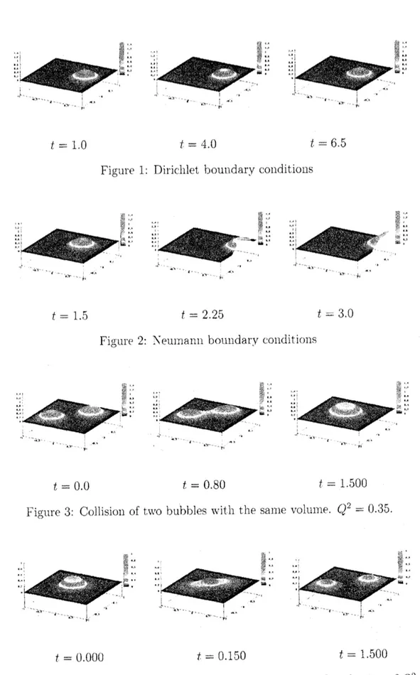
The
first example is
calculated
under
Dirichlet boundary
conditions
and
$Q^{2}=0.35$
.
An
initial
velocity is
imparted
to the bubble. It approaches the boundary
of
$\Omega$,
reflects
$\mathrm{O}11$$\mathrm{t}1_{\mathrm{I}}\mathrm{e}$
boundary
and
stops
in
a
certain
position.
The second example
uses
Neumann boundary
conditions
and
$Q^{2}=0.35$
.
$\mathrm{I}_{11}$this
case, after
$\mathrm{t}\mathrm{o}\mathrm{u}\mathrm{c}\mathrm{h}\mathrm{i}_{1\mathrm{l}}\mathrm{g}$the
boundary,
the bubble
moves
along
the
boundary.
The
bubble
stops
and
keeps
$\mathrm{t}1_{1}\mathrm{e}$smallest
surface
when
reaching the
corner
of
$\Omega$.
The third
example
treats acollision of two
bubbles
with the
same
volume. After
the collision,
the bubbles merge.
In the last
example
we
set
$Q^{2}=0.03(x_{1}x_{2}>0)$
alld
$Q^{2}=0.35$
otherwise. The
value of
$Q^{2}$
determines
the
contact angle
on
the free boundary according to the free
boundary
condition.
Therefore, the bubble lies down if
$Q^{2}$
distribution becomes small
$f=1.0$
$t=4.0$
$f=6.5$
Figure 1: Dirichlet
boundary
conditions
$f=1.5$
$t=2.25$
$t=3.0$
Figure 2:
$-\backslash ^{\tau}\mathrm{e}\mathrm{U}1\mathrm{n}\mathrm{a}\mathrm{n}11$boundary
$\mathrm{C}^{\cdot}O11\mathrm{d}\mathrm{i}\mathrm{t}\mathrm{i}\mathrm{o}11_{\iota}\mathrm{S}$$t=0.0$
$t=0.80$
$t=1.500$
Figure
3: Collision
of
$\mathrm{t}\iota\iota’ \mathrm{o}$bubbles
with
the
sal1le
$\mathrm{v}\mathrm{o}1_{\mathrm{U}111\mathrm{t}^{\supset}}$
.
$Q^{2}=\mathrm{t}\mathrm{I}.35$
.
$t$
$=0.000$
$t=0.150$
$t=1.500$
$\mathrm{F}\mathrm{i}_{\mathrm{t}\supset}(f\mathrm{u}\mathrm{r}\mathrm{e}$
$4$
:The
bubble
is
divided
to
$\mathrm{t}\mathrm{v}^{\gamma}\mathrm{o}$ $\mathrm{b}_{\iota}\mathrm{v}$
the
llon-Ulliforln
distribution of
6
Conclusions
Anumerical method
for
a
bubble motion
with
free
boundary and
$\mathrm{v}\mathrm{o}\mathrm{l}\mathrm{u}\mathrm{m}\mathrm{e}$constraint
was
developed.
The model
equation
beconles
free
boundary
$\mathrm{p}\mathrm{r}\mathrm{o}\mathrm{b}\mathrm{l}\mathrm{e}\ln$of degellerate
hyperbolic type
which is
diffcult
to treat. We have introduced
a
variational method to
solve tl
$\mathrm{l}\mathrm{i}\mathrm{s}$$\mathrm{p}\mathrm{r}\mathrm{o}\mathrm{b}\mathrm{l}\mathrm{e}\ln$
alld
it
gives good lmlllerical results.
This
model
can
also be
applied
to
the nlotioll of
oil
on
the
$\mathrm{b}\mathrm{o}\mathrm{t}\mathrm{t}\mathrm{o}\iota 11$of
water
or
to proble
$\mathrm{m}\mathrm{s}$
related
to
the pllen0lnen0ll
of
a
water-drop
$\mathrm{d}\mathrm{r}\mathrm{i}\mathrm{p}\mathrm{p}\mathrm{i}_{1\mathrm{l}}\mathrm{g}$from
$\mathrm{c}\mathrm{e}\mathrm{i}1\mathrm{i}_{11_{5}^{\mathrm{O}}}.$.
Therefore,
this work has
lllally
applications
and is significant for the
future studying of hyperbolic free
boundary
problelns.
It
is
reported
about the
former example that the gradient of temperature,
wetness or
areal
density
of surface activator makes oil droplet
run on
the
$\mathrm{b}\mathrm{o}\mathrm{t}\mathrm{t}\mathrm{o}\ln$plane
and
the droplet
repeats
the division and
union while moving
(see
[10]).
And
we are now
involved in
the
development
of numerical algorithm which describes
the
division and union
$\mathrm{o}\mathrm{f}_{1}\mathrm{n}\mathrm{u}1\mathrm{t}\mathrm{i}\mathrm{p}1\mathrm{e}$bubbles.
References
[1]
H. W. Alt
-L.
A.
Caffarelli,
.,‘Existence
and
$regular\dot{\iota}\mathrm{f}y$
for
o
$m\mathrm{i}nz\uparrow num$
problem
with
free
boundary”,
J. Reine Angew.
Math.,
325
(1981), 105-144,
[2]
H.Berestycki
- $\mathrm{L}.\mathrm{A}.\mathrm{C}\mathrm{a}\mathrm{f}\mathrm{a}\mathrm{f}\mathrm{i}^{\backslash }\mathrm{e}11\mathrm{i}$-
L.Nirenberg,
a
Uniform
e
stimates
for
regularization
of free
boundary problems
”,
in Analysis
and
Partial Differential
Equation, Marcel
Dekker,
New
York,
1990.
[3]
M.
Giaquinta,
.
multiple integrals
in the
calculus
of
variations
and
nonlinear
el-$l\iota pt\mathrm{i}c$
s
ystems”,
$\mathrm{P}\mathrm{r}\mathrm{i}\mathrm{n}\mathrm{c}\mathrm{e}\mathrm{t}_{011}$University Press,
1983.
[4] H.
Imai
- $\mathrm{I}\iota^{r}$.
Kikuchi
-K.
Nakane
-S. Omata
-T.
Tachikawa,
“A
numerical
approach
to
the
asymptotic behavior
of
solutions
of
a one-iirnensional
hyperbolic
free
boundary
problem”, JJIAM 18
No.1(2001)\43-58.
[5]
$\mathrm{I}^{\mathrm{s}_{\llcorner}^{r}}$.
Kikuchi
-S.
Omata,
”A
free
boundary problem
for
a
one
dimensional hyperbolic
equation”,
Adv.
Math.
Sci.
Appl. 9 No.2
$(1999)\dot,$
775-786.
[6]
0.
$\mathrm{L}\mathrm{a}\mathrm{d}\mathrm{y}\mathrm{z}\mathrm{h}\mathrm{e}\mathrm{n}\mathrm{s}\mathrm{k}\mathrm{a}_{\iota}\mathrm{y}\mathrm{a}$ -N. Uraltseva,
”Linear and
Quasilinear Elliptic Equations J’,
Acade
mic Press, New York and
London,
1968.
[7] T.
$\mathrm{N}\mathrm{a}_{5}\sigma \mathrm{a}\mathrm{s}\mathrm{a}\backslash \mathrm{v}\mathrm{a}$ - $\mathrm{I}\mathrm{c}^{r}$.
Nakane
-S.
Omata, “Numerical Computations
for
$mot\dot{\iota}on$
of
vortices governed by a Hyperbolic
Ginzburg-Landau
System”, Nonlinear Anal. 51
(2002)
No.l
Ser
A: Theory Methods,
67-77.
[8]
S.
Omata,
‘\prime A
Numerical
treatment
offilm
$mot_{i}on$
with
free
boundary”,
Adv. Math.
$\mathrm{S}_{\mathrm{C}\grave{1}}$