- 11 - 2009 IEEE Workshop onNonlinear Circuit Networks, Tokushima, Dec 11-12, 2009

Multi-Layer Perceptron with Chaos Glial Network

Chihiro Ikuta

Dept. of Electrical and Electronic Eng., Tokushima University

Email: [email protected]

Yoko Uwate Institute of Neuroinfomatics,

University / ETH Zurich, [email protected]

Yoshifumi Nishio

Dept. of Electrical and Electronic Eng., Tokushima University

[email protected]

I. I

Back Propagation (BP) was introduced by Rumelhart in 1986 [1]. BP is used for learning algorithm of MLP and the error propagates backwards in the network. MLP using BP al- gorithm is well known to perform for the pattern classification tasks. However, the solution of the network often falls into the local minimum, because BP uses the steepest descent method for the leaning process. Generally, if the solution of MLP falls into the local minimum, it can not escape. In order to avoid this problem, some methods to release the solution from the local minimum are required.

In this study, we propose a chaos glial network which connects to MLP. We consider that glial cells produce chaotic oscillation which is affected to neurons. This view is motivated by investigations of the Hopfield network solving combi- natorial optimization problems with the help of a chaotic input signal component, designed in order to avoid local minima. It appears, from computer simulations, that a chaotic input component may substantially enhance the capability of avoiding these local minima [2]-[4]. Hence, we believe that chaotic signals may be used to further enhance the efficiency of the proposed chaos glia neural network.

Furthermore, chaotic oscillation generated from glial cells propagates to the neighbor glial cells. Namely, certain neuron in this network is affected from some of glial cells located at a nearby site. We apply the proposed MLP with chaos glial network for solving Two-Spiral Problem (TSP) and confirm the efficiency by computer simulations.

II. M

-L

P

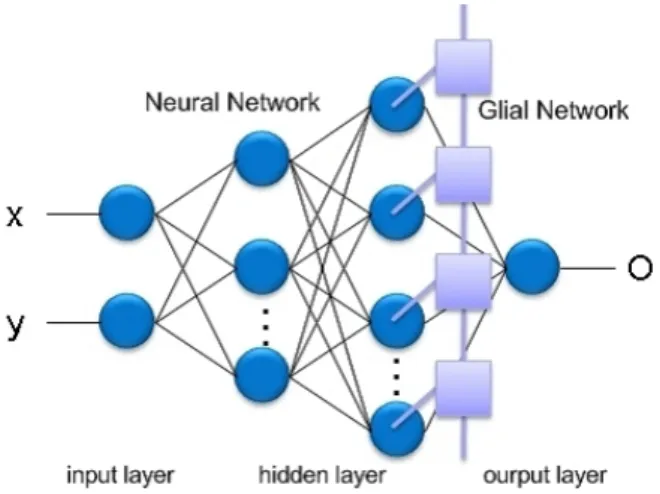
MLP is a most famous feed forward neural network. This network is used for pattern recognition, pattern classification, and other tasks. MLP has some layers, it has mainly input layer, hidden layer, and output layer. Generally, it is known that MLP can solve a more difficult task if the number of layer or neuron is increased. We consider MLP which is composed of four layers (one input layer, two hidden layers and one output layer), and MLP has the chaos glial network in the second layer of the hidden layer. The proposed MLP with the chaos glial network structure (connected 2-20-40-1) is shown in Fig. 1.

A. Neuron Updating Rule

The updating rule of neurons in the input layer, the first hidden layer and the output layer is described by Eq. (1) which

Fig. 1. MLP with chaos glial network.

is conventional updating rule.

x

(t + 1) = f



 ∑

j=1

w

(t)x

(t) − θ

(t)



 , (1)

In the chaos glial neural network, chaotic oscillation is added to neurons in the second hidden layer. This neuron’s updating rule is following as Eq. (2).

x

(t + 1) = f



 ∑

j=1

w

(t)x

(t) − θ

(t) + αΨ

(t)



 ,(2) where x : input or output, w : weight parameter, θ : threshold, ψ, Ψ : chaotic oscillation, α : amplitude of chaos and f : output function. And we use sigmoid for the output function as Eq. (3).

f (a) = 1

1 + e

, (3)

In the biological neural network, it is known that the glial cells affect to the neighbor neurons over a wide range by propagating in the network [6]. In order to realize this phenomena, we add chaotic oscillation to neurons by using Eq. (4).

Ψ

(t) =

∑

β

ψ

(t), (4)

Nonlinear Circuit Networks, Tokushima, Dec 11-12, 2009

- 11 -

where β denotes attenuation parameter and k is the prop- agating range in the glial network. Chaotic oscillation is propagating in the glial network.

III. C

O

G

N

We use skew tent map to generate chaos. This map is one of simple chaotic maps and the center of map is shifted for a little from the standard tent map. This chaotic map is defined by Eq. (5). Neurons in the second hidden layer are affected chaotic oscillation by Eq. (5) into the Eq.(4).

ψ

(t + 1) =

{

1+A

( − 1 ≤ ψ(t) ≤ A)

−2ψ(t)+1+A

1−A

(A < ψ(t) ≤ 1)

, (5)

Here, we consider the case that we prepare two similar initial values of chaos map for adding two adjacent neurons. Figure 2 shows the two time series obtained from the skew tent map when initial values are fixed as ψ

(0) = 0.12560 and ψ

(0) = 0.12561. From this figure, the plots of the two time series

Fig. 2. Time Series of Skew Tent Map.

are spread and difference between two time series becomes large with time, even if we use similar initial value to generate chaos. This is typical phenomena of chaos known as butterfly effect. If glial cells add these chaos to neurons, each neuron is affected with a completely different oscillation.

However, in the real biological neuro-glial network, glial cells affect each other with neighbor cells. We use the chaos glia propagating equation (Eq. 4) for having correlation each other of neighbor glial cells. Figure 3 shows two chaotic time series by using Eq. (4). The parameters are fixed as β = 0.8, m = 5. Two chaotic time series have similar peek points. We consider that these chaotic time series have some correlations.

IV. S

In this section, the difference in the performance of our MLP; MLP with chaos glial network and the conventional MLP is compared.

Fig. 3. Time Series of Skew Tent Map with Correlation.

A. Two-Spiral Problem

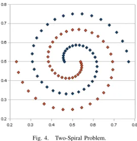
We apply the proposed network for solving TSP [5]. MLP learns to each point of two spirals, and MLP learns by using BP algorithm. Each MLP learns the two spirals by setting up

Fig. 4. Two-Spiral Problem.

same weights before learning process. We prepare 98 data of two spirals as shown in Fig. 4. The number of learning points is fixed as 500000. We investigate the error which is modified in the meantime. The error function is defined as Eq. (6).

E = 1 n

∑

| t

− O

| , (6) where E : error value t : target value, O : output value.

B. Changing the number of neuron adding chaos

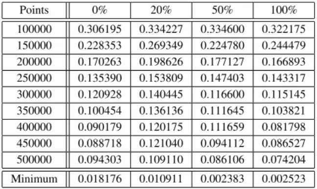
We investigate the learning ability when the number of neuron adding chaos is changed. In this simulation, we add chaos to the neurons in the second hidden layer’s. We change the percentage of neuron adding chaos as follows 0%, 20%, 50%, and 100%. The simulation result is summarized in Tab. I.

From Tab. I, we obtain the best learning ability when all neu- rons in the second hidden layer are added chaotic oscillation.

- 12 -

TABLE I

THEPERFORMANCE OFMLPWITHCHAOSGLIALNETWORK BY CHANGING THENUMBER OFNEURONADDINGCHAOS

Points 0% 20% 50% 100%

100000 0.306195 0.334227 0.334600 0.322175 150000 0.228353 0.269349 0.224780 0.244479 200000 0.170263 0.198626 0.177127 0.166893 250000 0.135390 0.153809 0.147403 0.143317 300000 0.120928 0.140445 0.116600 0.115145 350000 0.100454 0.136136 0.111645 0.103821 400000 0.090179 0.120175 0.111659 0.081798 450000 0.088718 0.121040 0.094112 0.086527 500000 0.094303 0.109110 0.086106 0.074204 Minimum 0.018176 0.010911 0.002383 0.002523

In the next simulation, we add chaotic oscillation to every neurons in the second hidden layer.

C. Results of Each MLP Learning

We compare MLP with chaos glial network, the conven- tional MLP and MLP with random glial network. In the ran- dom glial network, glial network produces random oscillation.

Each result is summarized in Tab. II.

TABLE II

THEPERFORMANCE BYUSINGEACHMLP Point Conventional Random Chaos 100000 0.274507 0.299191 0.265852 150000 0.189218 0.228571 0.191319 200000 0.142849 0.165421 0.151007 250000 0.111989 0.136988 0.118951 300000 0.084422 0.118154 0.099801 350000 0.093832 0.098092 0.088131 400000 0.081747 0.086327 0.077735 450000 0.079630 0.087916 0.071450 500000 0.076502 0.083399 0.068681 Minimum 0.0125310 0.0104630 0.0072510

At start learning, conventional MLP is better than the others.

However, after 300000 learning points MLP with chaos glial network gains better performance than the conventional MLP.

MLP with random glial network shows the most worst result.

If we focus on the minimum error, MLP with chaos glial network can find smallest error value. Because similarity of near neurons performs well by effects of chaos glial cells. And when MLP falls into local minima, chaos helps to escape with effectively.

Figure 5 is a typical example of learning curve. MLP with random glial network can not learn to two spirals. MLP with chaos glial network and the conventional MLP can learn to it, and the chaos glial network converges to the lower error value.

The learning curve of the conventional MLP is smooth. While, the others have little vibration. We consider that this vibration phenomena makes to escape out from the local minimum.

Fig. 5. The Error Curve by Three MLP Networks.

V. C

In our study, we have proposed a chaos glial network. This network gave chaotic oscillations to the second hidden layer’s neuron and this chaotic oscillation propagates to other neurons.

We confirmed that MLP with chaos glial network gains better performance than the conventional MLP and into MLP with random glial network for solving TSP.

R

[1] D.E. Rumelhart, G.E. Hinton, and R.J. Williams, “Learning representa- tions by back-propagating errors,”Nat., vol.323-9, pp.533-536, 1986.

[2] Y. Hayakawa, A. Marumoto, and Y. Sawada, “Effects of the chaotic noise on the performance of a neural network model for optimization problems,”

Phys. Rev. E, vol. 51, no. 4, pp. 2693-2696, Apr. 1995.

[3] T. Ueta, Y. Nishio, and T. Kawabe, “Comparison between Chaotic Noise and Burst Noise on Solving Ability of Hopfield Neural Networks,”Proc.

NOLTA’97, vol. 1, pp. 409-412, Nov. 1997.

[4] Y. Uwate, Y. Nishio, T. Ueta, T. Kawabe, and T. Ikeguchi, “Performance of Chaos and Burst Noise Injected to the Hopfield NN for Quadratic Assignment Problems,”IEICE Transactions on Fundamentals, vol. E87- A, no. 4, pp. 937-943, Apr. 2004.

[5] J.R. Alvarez-Sanchez, “Injecting knowledge into the solution of the two- spiral problem,”Neural Comput. & Applic., vol.8, pp.265-272, 1999.

[6] S. Koizumi, M. Tsuda, Y. Shigemoto-Nogami, and K. Inoue, “Dynamic inhibition of excitatory synaptic transmission by astrocyte-derived ATP in hippocampal cultures,”Proc. Natl. Acad. Sci. U. S. A, vol.100, pp.11028- 11028, 2003.

- 13 -