ResourceandNetworkManagementFrameworkforaLarge-ScaleSatelliteCommunicationsSystem PAPER

(1)

PAPER

Resource and Network Management Framework for a Large-Scale Satellite Communications System

Yuma ABE^†,††a),Member, Masaki OGURA^†††,Nonmember, Hiroyuki TSUJI^†,Senior Member, Amane MIURA^†,Member,andShuichi ADACHI^††,Nonmember

SUMMARY Satellite communications (SATCOM) systems play important roles in wireless communication systems. In the future, they will be required to accommodate rapidly increasing communication requests from various types of users. Therefore, we propose a framework for efficient resource management in large-scale SATCOM systems that integrate multiple satellites. Such systems contain hundreds of thousands of communication satellites, user terminals, and gateway stations; thus, our proposed framework enables simpler and more reliable communication between users and satellites. To manage and control this system efficiently, we formulate an optimization problem that designs the network structure and allocates communication resources for a large-scale SATCOM system. In this mixed integer programming problem, we allow the cost function to be a combina- tion of various factors so that SATCOM operators can design the network according to their individual management strategies. These factors include the total allocated bandwidth to users, the number of satellites and gateway stations to be used, and the number of total satellite handovers. Our numerical simulations show that the proposed management strategy outperforms a conventional strategy in which a user can connect to only one specific satellite determined in advance. Furthermore, we determine the effect of the number of satellites in the system on overall system performance.

key words: satellite communications, large-scale system, resource man- agement, network design problem, time-varying network

1. Introduction

There has been a gradual increase in the demand for satellite communications (SATCOM) in recent years. The total capacity demand for high-throughput SATCOM systems is expected to increase further at an average rate of approximately 32% from 2014 till 2023[1]. Furthermore, it is estimated that SATCOM systems are required to achieve Tbps-class throughput by early 2020s[2]. To meet this demand in the near future, SATCOM systems will be developed as large- scale satellite constellation systems designed to achieve various communication objectives through the cooperation and coordination of multiple integrated satellites[3], [4]. Re- cently, several companies have initiated the construction of global communication networks by launching hundreds of thousands of communication satellites into space[5],[6].

Manuscript received June 20, 2019.

Manuscript revised September 21, 2019.

†The authors are with Space Communications Laboratory, Wireless Networks Research Center, National Institute of Infor- mation and Communications Technology, Tokyo, 184-8795 Japan.

††The authors are with the Graduate School of Science and Technology, Keio University, Yokohama-shi, 223-8522 Japan.

†††The author is with the Division of Information Science, Nara Institute of Science and Technology, Ikoma-shi, 630-0192 Japan.

a) E-mail: [email protected] DOI: 10.1587/transfun.2019EAP1088

These networks will involve collaboration between geostationary earth orbits (GEOs) and non-geostationary earth orbits (NGEOs) that orbit at different altitudes; e.g., low and medium earth orbits (LEOs and MEOs)[7]. Furthermore, the integration of SATCOM systems and the fifth generation mobile communication system (5G) is currently in progress[8],[9], which aims to not only increase the communication capacities of the system but also accommodate various types of communication requests arising from emerging information technologies such as the Internet of Things (IoT) and the Internet of Everything (IoE).

In current SATCOM systems, a lack of available satellites means that each user typically connects to only one specific satellite determined in advance; this is termed a conventional non-integrated system. However, future large- scale SATCOM systems should allow users to connect with several candidate satellites; this is termed an integrated system. Furthermore, the operators of future SATCOM systems will have to accommodate time-variability within the system components, such as the number of users, amount of communication requests, availability of satellites, and propagation environments. Therefore, a framework is required for the efficient design and resilient operation of future large- scale SATCOM systems, for which the current management methodology does not necessarily apply.

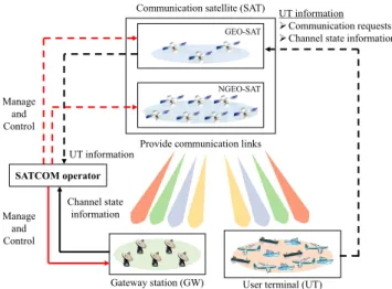
In this study, we focus on the large-scale SATCOM system illustrated in Fig. 1. This system includes communication satellites (SATs), user terminals (UTs) such as aircraft

Fig. 1 Schematic of the large-scale SATCOM system used in this study.

This system includes communication satellites (SATs), user terminals (UTs), gateway stations (GWs), and a SATCOM operator which manages and controls the SATs and GWs. In this system, available SATs, the amount of UT requests, and the state of propagation environment fluctuate.

(2)

and ships that request communication links, and gateway stations (GWs) connected to the ground network. A SAT- COM operator manages and controls the SATs and GWs to provide communication links to the UTs based on their requests. The bidirectional communication links between SATs and UTs are termed user links (ULs) and the links between SATs and GWs are termed feeder links (FLs). To establish a SATCOM network, it is important to appropri- ately allocate communication resources such as bandwidth to the ULs and FLs.

Furthermore, time-variability in the amount of UT requests and in the propagation environment of the ULs and FLs can cause fluctuations in the amount of required resources provided by the SATs and GWs. Thus, static allocation of resources can result in network disconnection and high latency. Therefore, it is important to allow the config- uration of the SATCOM system to change dynamically so that the SAT resources can be fully and efficiently utilized in the presence of hundreds of thousands of SATs, UTs, and GWs. To achieve this goal, the SATCOM operator should be able to flexibly adapt the SATCOM network structure. When designing a time-varying SATCOM network[10], frequent satellite handovers can be expected, whereby the UTs and GWs change which SAT is connected over time, which can lead to wasteful power consumption. However, the operator can avoid these handovers by utilizing an appropriate cost function. We term the resulting network a flexible SAT- COM network. In this study, we propose a framework for designing such a flexible network in a large-scale SATCOM system.

Network design problems have been investigated in many areas [11] including communication networks [12], power networks[13], transportation networks[14], and supply chain networks[15]. Although previous literature has reported various frameworks for the operation of SATCOM systems (see, e.g.,[16]–[18]), few studies have considered the time-varying UT requests in a large-scale network. Con- versely, our novel method adapts the large-scale SATCOM system by establishing a flexible network to cope with time- varying UT requests.

In the proposed method, we first describe the network structure of UL and FL in terms of network connection matrices. In terms of the matrix elements, we describe the constraints in the network design. We then describe candidate cost functions, including the sum of allocated bandwidths for the UT, the number of active SATs and GWs, and the number of satellite handovers. The SATCOM operator can then define their desired cost function by combining the candidate functions according to their individual management strategy. Using these constraints and cost functions, we formulate the SATCOM network design problem as a mixed integer programming problem. This formulated optimization problem is solved to simultaneously obtain the resource allocation and network structure.

The proposed framework enables us to consider different types of SATs in a unified manner. In this formulation, we define sets of connectable pair candidates in UT-SAT

and SAT-GW links. By incorporating these sets into the optimization problem, various types of SAT can be distin- guished such as satellite orbit (e.g. GEO and NGEO), beam width (e.g. wide and narrow spot beam), and power SAT.

This method constructs an efficient SATCOM network that efficiently utilizes limited resources. As a result, UTs can obtain the resources as they request, and the SATCOM operator can make the flexible SATCOM network more reliable.

The originality of this study lies in the fact that the proposed method allows managing and controlling multiple GEO and NGEO satellites in a unified manner, and it helps cope with the time-varying UT requests by constructing the flexible SATCOM network.

The remainder of this paper is organized as follows. In Sect. 2, we present the model of the large-scale SATCOM system integrating multiple SATs, UTs, and GWs to design a flexible network. In Sect. 3, we formulate the optimization problem to obtain the resource allocation and network structure as a mixed integer programming problem. In Sect. 4, the effectiveness of the proposed method is verified using numerical simulations with three examples. Finally, we present our conclusions and suggest future research in Sect. 5.

2. Large-Scale SATCOM System

In this section, we present our model of the large-scale SAT- COM system integrating multiple SATs, UTs, and GWs.

2.1 System Architecture

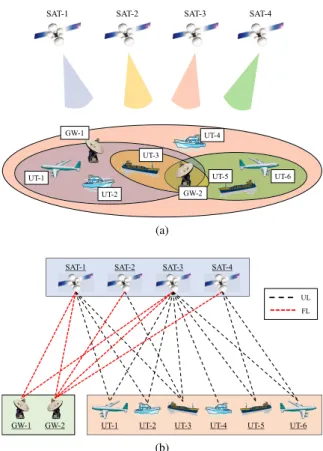
This study focuses on the SATCOM system architecture illustrated in Fig. 2.

In this large-scale SATCOM system, the UTs have several candidates for SATs to connect. The SATs are divided into two different types: GEO-SAT and NGEO-SAT. GEO- SATs have a larger bandwidth and wider beam coverage than the NGEO-SATs, whereas the number of SATs that can

Fig. 2 Architecture of the large-scale SATCOM system. Solid and dashed lines represent wired and wireless communication links, respectively. Red lines represent the actions of the SATCOM operator.

(3)

be placed at the GEO is limited and the launching cost is high. NGEO-SATs can perform lower latency communication than GEO-SATs; however, multiple NGEO-SATs must be launched for global coverage [19]. Thus, integrating GEO-SATs and NGEO-SATs brings a variety of advantages;

for example, UTs are able to obtain more bandwidth than ever.

As a specific feature of this system, these integrated SATs work as repeaters of communication signals, whereas the GEO-SATs also work as aggregators of UT information such as communication requests and channel state information of the ULs. We assume that this aggregation function is installed in all GEO-SATs; that is, each UT must be able to connect to at least one GEO-SAT to transmit the UT information.

The SATCOM operator works as a controller of this system by managing and controlling their SATs and GWs.

The SATCOM operator aggregates the UT information via the GEO-SATs and channel state information of FLs from the GWs. Based on the aggregated information, the operator then determines the resource allocation and network structure using the method proposed in Sect. 3. Then, the SATs provide communication links to the UTs and the SATCOM network is established.

2.2 System Description

The large-scale SATCOM system consists of multiple UTs, SATs, and GWs labeled by the index sets N_U = {1,2, . . . ,N_U},N_S = {1,2, . . . ,N_S}, and N_G = {1,2, . . . ,N_G}, respectively. Throughout this paper, we use the indicesi,j, and` to denote UTs, SATs, and GWs, respectively. The maximum bandwidths of SAT-j and GW-`

are denoted byB_S^j ≥0 and B_G^` ≥0, respectively. For each timek ≥0, each UT sends a communication request to any SAT; the amount of the communication request from UT-iis denoted bydⁱ_k ≥0.

We place the following assumptions on the SATCOM system.

Assumption 1. Each UT can connect to up to one SAT. Each SAT can connect to up to one GW.

Assumption 2. SATs have no inter-satellite links.

For UT-SAT and SAT-GW pairs, we define the following connectable candidate sets.

Definition 1. The sets of connectable pair candidates in UT- SAT and SAT-GW links at timekare defined as

A^US

k :={(i,j)∈ N_U× N_S |UT-iand SAT-jcan be connected at timek.} ⊆ N_U× N_S, (1a) A^SG

k :={(j, `)∈ N_S× N_G|SAT-jand GW-`can be connected at timek.} ⊆ N_S× N_G, (1b) respectively.

We assume that setsA^US

k andA^SG

k are known by the

Fig. 3 (a) Example of the SATCOM system. (b) Connectable pair candidates in UT-SAT and SAT-GW links derived from (a), where black and red dot lines represent the connectable candidateA^US

k andA^SG

k , respectively.

SATCOM operator in advance and are determined indepen- dently of the link budget requirements[20]. The sets change over time due to time-variability in the satellite position and propagation environment. For example, because NGEO- SATs rotate around the earth periodically on a prescribed orbit, the operator can determine the sets in advance. Note that, during operation of the SATCOM system, the operator can update the sets using channel state information from the UTs and GWs.

Figure 3(a) shows an example of the SATCOM system at time k. Suppose thatN_U =6,N_S =4, andN_G =2 and each SAT forms a different shape and size of the beam. In Fig. 3(b), the candidate sets of UT-SAT and SAT-GW pairs are illustrated as a graph. In this example,A^US

k andA^SG

k are

represented by A^US

k ={(1,1),(1,3),(2,1),(2,3),(3,1),(3,2), (3,3),(4,3),(5,3),(5,4),(6,3),(6,4)}, A^SG

k ={(1,1),(1,2),(2,2),(3,1),(3,2),(4,2)}.

The UT-SAT and SAT-GW pairs to be connected are chosen from these candidates.

3. Problem Formulation

In this section, we present design variables and constraints and define cost functions relevant to the SATCOM system.

(4)

Then, we formulate the optimization problem to determine the resource allocation and network structure for the large- scale SATCOM system.

The following notational conventions are used. Sym- bolsR,Rⁿ,R^n×m, and{0,1}^n×mdenote the sets of real numbers,n-dimensional real vectors, n×mreal matrices, and n×mbinary matrices, respectively.

3.1 Design Variables and Constraints

In this subsection, we describe the design variables and constraints of our network optimization problem.

The amount of bandwidth that the operator plans to allocate to the UTs is denoted by

xk =f

x¹_k x²_k · · · x_k^N^U g>

∈R^N^U, where

xⁱ_k ≥0, ∀i∈ N_U (2)

represents the allocated bandwidth to UT-i. Here, we assume that the following inequality holds:

xⁱ_k ≤dⁱ_k, ∀i∈ N_U, (3) which means that the allocated bandwidth cannot be more than each UT request^†.

The links of the SATCOM network that the operator plans to design are represented by the following network connection matrices. The matrices for UT-SAT and SAT-GW links at timekare denoted by Ck =[c_k^j,i]j,i ∈ {0,1}^N^S^×N^U andEk =[e^`,j_k ]`,j ∈ {0,1}^N^G^×N^S, respectively. The element c_k^j,i is 1 for a connected UT-i and SAT-j and 0 otherwise;

similarly, e^`,_k^j is 1 for a connected SAT-j and GW-`and 0 otherwise:

c_k^j,i ∈ {0,1}, ∀(i,j)∈ A^US_k , (4a) e^`,j

k ∈ {0,1}, ∀(j, `)∈ A^SG

k . (4b)

According to Assumption 1, we have X

j:(i,j)∈ A^US_k

c_k^j,i ∈ {0,1}, ∀i ∈ N_U, (5a) X

`:(j,`)∈ A^SG_k

e^`,_k^j ∈ {0,1}, ∀j ∈ N_S. (5b)

These constraints are equivalent to the following inequality constraints:

X

j:(i,j)∈ A^US_k

c_k^j,i ≤1, ∀i∈ N_U, (6a) X

`:(j,`)∈ A^SG k

e^`,_k^j ≤1, ∀j∈ N_S (6b)

†This is a technical constraint required to solve the optimization problem efficiently. In a real system, the allocated bandwidth can be more than the UT request.

because a feasible set of constraints in (6) is equivalent to that of the original constraints in (5) under the binary variables c_k^j,iande^`,_k^j.

We represent the amount of bandwidth allocated to each link by resource flow matrices defined asYk ∈R^N^S^×N^Uand Zk ∈R^N^G^×N^Sfor UT-SAT and SAT-GW links, respectively.

We define the elements of these matrices as y^j,i

k =(

xⁱ_k, (i,j)∈ C_k,

0, otherwise, (7a)

z^`,_k^j =







 X

i:(i,j)∈ Ck

y_k^j,i, (j, `)∈ E_k,

0, otherwise, (7b)

whereC_k andE_kare defined as C_k :={(i,j)∈ A^US

k |c_k^j,i=1}, (8a)

E_k :={(j, `)∈ A^SG_k |e^`,j_k =1}, (8b) respectively. According to these definitions, y^j,i

k andz^`,^j

k in (7) are linear inxⁱ_k whenCk andEk are given.

We require that the following capacity constraints hold:

X

i:(i,j)∈ Ck

y_k^j,i ≤B_S^j, ∀j ∈ N_S, (9a)

X

j:(j,`)∈ Ek

z^`,_k^j ≤B^`_G, ∀` ∈ N_G. (9b)

To ensure full and efficient use of resources, our network is designed to conserve the in- and out-flow of each link.

Thus, we require that the following conservation laws hold true:

xⁱ_k = X

j:(i,j)∈ Ck

y_k^j,i, ∀i∈ N_U, (10a) X

i:(i,j)∈ Ck

y_k^j,i = X

`:(j,`)∈ E_k

z^`,_k^j, ∀j ∈ N_S. (10b)

3.2 Cost Functions

In this subsection, we introduce candidate factors for the cost function to ensure a cost-efficient and flexible design of our SATCOM system. These candidates also include management strategy factors related to the SATCOM operator.

1.UT utility factor: The first factor measures the utility of the UTs and is defined as follows:

X

i∈NU

xⁱ_k. (11)

Maximizing this factor increases the total allocated bandwidth to the UTs.

2.SAT and GW operations factor: The second factor measures the number of active SATs and GWs to be used. We denote the number of active SATs and GWs at each timek as ˆN_S,k and ˆN_G,k, respectively.

For ˆNS,k and ˆNG,k, the following lemma holds.

(5)

Lemma 1. Under Assumption 1, the numbers of active SAT and GW are represented by

Nˆ_S,k =rank(Ck), (12a)

Nˆ_G,k =rank(E_k), (12b)

respectively.

Proof. The number of active SATs and GWs at each time k is represented by the number of row vectors of C_k and Ek, respectively, where all elements are not zero. As c_k^j,i and e^`,j_k are binary variables, the row vectors of Ck and E_k are linearly independent because these vectors are not identical. Therefore, the number of active SATs and GWs is represented by that of linearly independent row vectors of Ck andEk; i.e., the rank ofCkandEk. Then, the equations

in (12) hold.

By minimizing the factors in (12), the UTs connect to as few SATs and GWs as possible. Therefore, the SATCOM operator profits because fewer active SATs and GWs reduce the operating costs of the system. By maximizing these factors, we can expect that network disconnection risks due to SAT and GW failures and propagation environment changes are reduced because the number of active SATs and GWs are increased and UT connections are distributed.

3.Handover factor: The third factor measures the number of satellite handovers. A time-varying network is also required to manage satellite handovers of UT-SAT and SAT-GW pairs.

We denote the numbers of satellite handovers of UT-SAT and SAT-GW pairs at each timekasn^US_k andn^SG_k , respectively.

Then, these numbers are represented by n_k^US= 1

2kCk−Ck−1k_F², (13a)

n_k^SG= 1

2kEk−Ek−1k_F², (13b)

respectively, wherekXk_Frepresents the Frobenius norm of a matrixX ∈R^n×mdefined by

kXk_F = vu t n

X

i=1 m

X

j=1

|x_{i j}|².

The factors in (13) directly represent the number of UT-SAT and SAT-GW pairs that change the connection. By minimizing these factors, we can ensure fewer frequent changes of the network and reduce the resulting power consumption. By maximizing these factors, we can make the network more se- cure and reduce wiretap risks because the network structure changes frequently.

Combining the factors in (11)–(13), we define the cost function at timekas

J_k =−w₁ X

i∈N_U

xⁱ_k+w_2srank(Ck)+w_2grank(Ek) +w_3skCk−Ck−1k_F² +w_3g kEk−Ek−1k_F², (14)

where w₁ ≥ 0, w_2s ∈ R, w_2g ∈ R, w_3s ∈ R, and w_3g ∈ R are the weights. The weightsw_2s, w_2g, w_3s, and w_3g can be negative when the corresponding factors are maximized. The SATCOM operator designs these weights according to their individual management strategy and can add other factors to the cost function as desired.

Remark 1. We assume that we can predict future UT requests and future connectable pair candidates^†. When we formulate an optimization problem in a model predictive control (MPC)[22]manner, the cost function at each time is defined by

J˜_k =

Tp

X

τ=1

J_k+τ,

whereTp denotes a finite-time prediction horizon. Here, the constraints must be satisfied across the entire prediction horizon. Using this approach to formulate the problem, we can obtain a solution to change the resource allocation and network structure in advance before the UT requests change.

3.3 Optimization Problem

In our network optimization problem, we attempt to find the following decision variables:

• Bandwidth allocation of UTs:x_k (a real vector)

• Network connection matrices of UT-SAT and SAT-GW links: Ck andEk (binary matrices)

• Resource flow matrices of UT-SAT and SAT-GW links:

YkandZk(real matrices)

We denote the solutions of these decision variables as ˆ

xk,Cˆk,Eˆk,Yˆk, and ˆZk.

Combining the cost function and constraints defined previously, we formulate the following network optimization problem.

Problem 1 (Network Optimization Problem). For a given N_U,N_S,N_G,B_S^j,B_G^`,A^US

k ,A^SG

k , andd_kⁱ, solve minimize J_k

subject to (2), (3), (4), (6), (7), (9), (10) to obtain ˆx_k,Cˆ_k,Eˆ_k,Yˆ_k, and ˆZ_k.

Problem 1 is a mixed integer programming problem because xk,Yk, and Zk are the real vector and matrices, whereas C_k and E_k are the binary matrices; i.e., the integer matrices. Although the mixed integer programming problem is NP-hard, this problem can be efficiently solved using the branch-and-cut algorithm, which is a heuristic algorithm[23]. Furthermore, optimization of the rank functions

†To obtain these future requests and connectable candidates, we have to predict future trends of UT requests and the propagation environment by analyzing past data. For example, UT requests can be effectively predicted using actual tracking data of UTs (see[21]).

(6)

in (12) is shown in Appendix.

Problem 1 is solved at every time instantkby the SAT- COM operator, who controls the SATCOM system described in Fig. 2. Using this result, the operator manages and controls SATs and GWs based on the obtained resource allocation and network structure.

4. Numerical Simulations

In this section, we conduct three numerical simulations to verify the performance of the proposed network design method in the integrated system. In Sect. 4.1, the basic performance of the proposed method is verified for simple static UT requests. In Sect. 4.2, we focus on dynamic UT requests and compare the performance of the proposed method in a system with integrated GEO-SATs and NGEO-SATs and in a conventional non-integrated system. In Sect. 4.3, we further verify the effect of the number of SATs in the system and compare the performance of integrated and non-integrated systems.

In these simulations, we assume that SATs use a different frequency band to prevent interference among communication links. To be consistent with this assumption, the UTs and GWs have an antenna to cover all the frequency bands utilized by the SATs. Furthermore, we ignore the influence of the propagation delay due to the propagation distance between UT-SAT and SAT-GW pairs.

To evaluate the performance of the method, we define the amount of bandwidth loss as

Lk = X

i∈NU

Lⁱ_k = X

i∈NU

max{0,dⁱ_k−xⁱ_k}, (15)

whereLⁱ_k represents the bandwidth loss of UT-iat each time k. Here, the bandwidth loss represents the total amount of the insufficient bandwidth required to meet UT requests.

The optimization problem is described by MATLAB YALMIP[24]and solved using the Gurobi Optimizer[25].

This solver implements the branch-and-cut algorithm to efficiently solve the mixed integer programming problem. These simulations are conducted using an Intel(R) Xeon(R) E5- 2687W CPU at 3.10 GHz with 64 GB RAM.

4.1 Example 1: Basic Performance Considering Static UT Requests

In this example, we focus on simple static UT requests in one step to confirm the basic performance of the proposed method. Assuming that all UT-SAT and SAT-GW pairs can be connected:

A^US=N_U× N_S, (16a)

A^SG=N_S× N_G. (16b)

The simulation parameters are shown in Table 1. We generate each UT requestdⁱ from a uniform distribution on [30,70] as follows:

Table 1 Simulation parameters for static UT requests.

NU NS NG B_S^j[MHz](∀j∈ N_S) B_G^`[MHz](∀`∈ N_G)

10 5 3 100 100

d=f

58 36 59 50 34 52 40 61 63 38 g>

. The cost function is defined as the total amount of bandwidth allocated to the UTs:

J=−X

i∈N_U

xⁱ,

wherew₁=1 and the other weights are set to 0 in (14).

The solutions obtained by solving Problem 1 were as follows:

ˆ x=f

41 36 59 50 34 30 40 0 10 0 g>

,

Cˆ=







0 0 0 1 0 0 1 1 1 1

0 0 0 0 0 0 0 0 0 0

0 1 0 0 1 1 0 0 0 0

0 0 1 0 0 0 0 0 0 0

1 0 0 0 0 0 0 0 0 0





 ,

Eˆ=







0 1 0 1 1

0 0 1 0 0

1 0 0 0 0





 ,

Yˆ =







0 0 0 50 0 0 40 0 10 0

0 0 0 0 0 0 0 0 0 0

0 36 0 0 34 30 0 0 0 0

0 0 59 0 0 0 0 0 0 0

41 0 0 0 0 0 0 0 0 0





 ,

Zˆ =







0 0 0 59 41

0 0 100 0 0

100 0 0 0 0





 .

The bandwidth lossLof each UT was L=f

17 0 0 0 0 22 0 61 53 38 g>

. Here, we set the simulation condition in order to satisfy inequalities in the total UT requests and total SAT and GW bandwidths:

X

i∈N_U

dⁱ (=491) ≤ X

j∈N_S

B_S^j (=500), X

i∈NU

dⁱ (=491)≥ X

`∈NG

B_G^` (=300)

held. Thus, all UT requests were not accommodated and the UTs only obtained a total of

X

i∈NU

ˆ xⁱ=300.

Therefore, the UT-8 and UT-10 did not obtain the bandwidths as ˆx⁸ = 0 and ˆx¹⁰ = 0 despite their connections to the SAT-1. By weighting each term xⁱ of the cost function, this unfairness can be avoided under this limited bandwidth situation.

4.2 Example 2: Comparison of Integrated and Non- Integrated Systems

In this example, we focus on dynamic UT requests that show

(7)

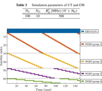
Table 2 Simulation parameters of SAT.

Type of SATs N_S B_S^j[MHz]

Visible period [steps]

(for each SAT)

GEO 5 500 -

NGEO group 1 24 250 5

65 (in total)

Table 3 Simulation parameters of UT and GW.

NU NG B_G^`[MHz](∀`∈ N_G)

100 10 500

Fig. 4 SAT visibility schedule. Over the visible period, the corresponding SATs can connect to all UTs and GWs.

temporal variability. The simulation parameters are shown in Tables 2 and 3 and the simulation is conducted inT =150 steps.

There is a total of 65 SATs in this SATCOM system, which is composed of five GEO-SATs and 60 NGEO-SATs divided into four groups. Figure 4 shows the SAT visibility schedule. Over a continuous visible period, the corresponding SATs can connect to all UTs and GWs. The GEO-SATs can be visible throughout the simulation time, whereas the visible period of the NGEO-SATs is limited to finite steps and repeated periodically. We assume that the period of the NGEO-SATs overlaps during two steps. The connectable pair candidate setsA^US

k andA^SG

k are obtained throughout the simulation time based on this schedule. Furthermore, the time-varying total SAT bandwidth is calculated from the bandwidthB_S^j of each SAT and this visibility schedule.

We assume that the SATs have beams with sufficient size to connect to all UTs and GWs when these SATs are in the visible period. The SATs have a steerable antenna to connect to multiple UTs and a fixed antenna to connect to the GWs. The UTs have a steerable antenna to track the SATs and the GWs have a sufficiently wide beam antenna to track all connected SATs. Furthermore, we assume that, when the visible period of multiple SATs overlaps in the same NGEO-SATs group, they can only connect to the same GW.

Fig. 5 Time-varying total UT requests (blue line) and total SAT and GW bandwidth (red and yellow lines, respectively).

The dynamics of the UT requests are described as dⁱ_k+1=γⁱ_kdⁱ_k, ∀i∈ N_U, (17) where the initial values of the UT request d₁ⁱ are generated from a uniform distribution on [10,30], and coeffi- cients γ_kⁱ are generated from a Gaussian distribution with N(1.0075,0.05)in each step.

Figure 5 shows the total time-varying UT requests, Pi∈NUdⁱ_k, and the total SAT and GW bandwidth: i.e., Pj:(i,j)∈ A^US_k ∩(j,`)∈ A^SG_k B_S^j andP

`∈N_GB_G^`, respectively. Ac- cording to this figure, the total UT requests exceed the total SAT and GW bandwidth at approximately k = 85 and k=120, respectively. The total GW bandwidth is larger than the total SAT bandwidth throughout the simulation time.

We define the cost function as J_k =− X

i∈NU

xⁱ_k+kC_k−C_k₋₁k²_F+kE_k −E_k−1k_F²,

wherew₁ =1,w_3s=w_3g=1, and the other weights are set to 0 in (14). Using this cost, we compare the following three methods: the method proposed for the integrated system that solves Problem 1 (Method A), a method to design a random network in the integrated system (Method B), and a method to design a random network in the conventional non-integrated system (Method C). In Methods B and C, the connection pairs (UT and GW to GEO-SAT or NGEO-SATs group) are determined randomly. In Method B, the pairs are determined at each time step and can be changed at the next step, whereas in Method C, the pairs cannot be changed throughout the simulation.

Due to the fixed connection pairs, the network structure C_kandE_k and the resource flowsY_kandZ_k are determined in advance. Thus, in Methods B and C, the bandwidth allocation ˆx_k is obtained by solving the following optimization problem:

minimize Jk

subject to (2), (3), (9), (10)

which is a linear programming problem becauseCk,Ek,Yk,

(8)

Fig. 6 Comparison of the performance of the proposed method in integrated and conventional non-integrated systems. Red, yellow, and blue lines represent the results of Methods A, B, and C, respectively.

andZk are given and the decision variable is onlyxk. Figure 6 shows the results of the bandwidth loss L_k among the three methods. The simulation was conducted using 30 trials for Methods B and C and the average bandwidth loss was utilized. Method A exhibited better performance than the other methods throughout the simulation time. Specifically, the bandwidth loss was almost zero during the interval fromk=1 to approximatelyk=85 because the total SAT bandwidth exceeded the total UT requests. In the other two methods, the bandwidth loss was not zero and the loss increased as the total UT requests increased because the GEO-SAT or NGEO-SATs group to which the UTs can be connected was limited. After the time instantk=85, the bandwidth loss of Method A also increased because the total UT requests exceeded the total SAT bandwidth. However, the average bandwidth loss of Method A was reduced by 58.5% fromk=85 to 150 compared to Methods B and C.

Furthermore, Method B exhibited worse performance than Method A, despite both methods involving the integrated system. This indicates that the performance is reduced by determining the network randomly, even when an integrated system is considered.

These results demonstrate the superior effectiveness of the proposed method in the integrated system compared to the conventional non-integrated system.

4.3 Example 3: Effect of the Number of SATs

In this example, we investigate the effect of the number of SATs by comparing the different performance of integrated and non-integrated system.

We assume that only GEO-SATs withB_S =500 MHz exist in the system and that all pairs can be connected as defined in (16). In this simulation, the number of GEO- SATs is increased from NS = 1 to 20. We set the cost function and the UT requests to be the same as Example 2 and the number of GWs and the GW bandwidth to NG = 20 and B_G = 500 MHz, respectively, so that an inequality Pj∈N_SB_S^j < P

`∈N_GB^`_G holds for any NS. Note that the

Fig. 7 Relationship between number of SATs and the time average of bandwidth loss. Red and blue lines represent the results of Methods A and C, respectively.

total SAT bandwidth ofN_S=14 to 20 exceeds the total UT requests throughout the simulation.

Figure 7 shows the result of bandwidth loss between the integrated (Method A) and non-integrated system (Method C). For the Method C simulation, the average bandwidth loss of 50 trials was utilized. In Fig. 7, the vertical axis represents the time average of the bandwidth loss throughout the simulation: (1/T)PT

k=1Lk.

This result indicates that the difference in performance depends on the number of SATs that exist in the system. For all N_S, the bandwidth loss of Method A was less than that of Method C. For a small number of satellites, the difference was small because the total SAT bandwidth was less than the UT request in both systems. However, the difference in bandwidth loss increased as the number of SATs increased with an average difference fromN_S =10 to 20 of approximately 530 MHz. Therefore, for a greater number of SATs, our proposed method in the integrated system exhibits better performance than the conventional non-integrated system.

Remark 2. In the integrated system, if all UTs can obtain a bandwidth equal to the UT request at timek, the following inequalities hold:

X

i∈N_U

dⁱ_k ≤ X

j∈N_S

B_S^j ≤ X

`∈N_G

B^`_G. (18)

However, in the non-integrated system, if all UTs can obtain a bandwidth equal to the UT request, the following inequalities hold:

X

i∈N_U^j

d_kⁱ ≤B_S^j, ∀j ∈ N_S and X

j∈N_S

B_S^j ≤ X

`∈N_G

B_G^`,

(19) where N^j

U ⊆ N_U is defined as a set of UTs connected to SAT-j.

According to these relationships, the inequalities in (18) hold if those in (19) hold, which means that all UTs can always obtain a bandwidth equal to the UT request in the

(9)

integrated system if this situation is achieved in the non- integrated system. This fact is proved easily by taking the sum of the former inequality in (19) withj ∈ N_S.

5. Conclusion

In this study, we proposed a framework for the efficient resource and network management of the large-scale SATCOM system integrating multiple SATs, UTs, and GWs. We formulated a network optimization problem to ensure efficient resource allocation and a network structure that can accommodate several UT requests, as well as improve the reliabil- ity of the flexible SATCOM network. In this framework, the SATCOM operator can design the network according to their individual management strategy by adjusting the weights of the cost function. The effectiveness of the proposed method in the integrated system was verified through numerical simulations, which proved that our proposed management strategy performed better than the conventional strategy. Fur- thermore, we determined the effect of increasing the number of satellites on the performance of the proposed and conventional strategies.

In future research, we aim to address the following research challenges for a large-scale SATCOM system:

• Site diversity

• Multi-satellite beamforming

• 5G-satellite integration

• Routing mechanism via inter-satellite links

• Flexible reconfigurable antenna

• Operations strategy

• Incentive mechanism

• Security

Acknowledgments

The first author acknowledges Mr. Hideaki Nakao from the University of Michigan for productive discussions on the problem formulation.

References

[1] Euroconsult, High Throughput Satellites: On Course for New Hori- zons, Euroconsult Executive Report, 2014.

[2] H. Hauschildt, C. Elia, H.L. Moeller, and J.M.P. Armengol, “Hy- dRON: High throughput optical network,” Proc. SPIE 10910, Free- Space Laser Communications XXXI, pp.109100K-1–9, 2019.

[3] Y. Hu and V.O. Li, “Satellite-based Internet: A tutorial,” IEEE Commun. Mag., vol.39, no.3, pp.154–162, 2001.

[4] L. Wood, A. Clerget, I. Andrikopoulos, G. Pavlou, and W. Dabbous,

“IP routing issues in satellite constellation networks,” Int. J. Satell.

Commun., vol.19, no.1, pp.69–92, 2001.

[5] J. Foust, “SpaceX’s space-Internet woes: Despite technical glitches, the company plans to launch the first of nearly 12,000 satellites in 2019,” IEEE Spectr., vol.56, no.1, pp.50–51, 2019.

[6] M. Harris, “Tech giants race to build orbital internet,” IEEE Spectr., vol.55, no.6, pp.10–11, 2018.

[7] J.N. Pelton and B. Jacque, “Distributed internet-optimized services via satellite constellations,” Handbook of Satellite Applications,

2nd ed., J.N. Pelton, S. Madry, and S. Camacho-Lara, eds., pp.249–

269, Springer, 2017.

[8] L. Boero, R. Bruschi, F. Davoli, M. Marchese, and F. Patrone, “Satel- lite networking integration in the 5G ecosystem: Research trends and open challenges,” IEEE Netw., vol.32, no.5, pp.9–15, 2018.

[9] R. Gopal and N. BenAmmar, “Framework for unifying 5G and next generation satellite communications,” IEEE Netw., vol.32, no.5, pp.16–24, 2018.

[10] P. Holme and J. Saramäki, “Temporal networks,” Physics Reports, vol.519, pp.97–125, 2012.

[11] R.K. Ahuja, T.L. Magnanti, and J.B. Orlin, Network Flows: Theory, Algorithms, and Applications, Prentice Hall, 1993.

[12] K. Xie, J. Cao, X. Wang, and J. Wen, “Optimal resource allocation for reliable and energy efficient cooperative communications,” IEEE Trans. Wireless Commun., vol.12, no.10, pp.4994–5007, 2013.

[13] L. Bahiense, G.C. Oliveira, M. Pereira, and S. Granville, “A mixed integer disjunctive model for transmission network expansion,” IEEE Trans. Power Syst., vol.16, no.3, pp.560–565, 2001.

[14] T.G. Crainic, “Service network design in freight transportation,” Eur.

J. Oper. Res., vol.122, no.2, pp.272–288, 2000.

[15] T. Santoso, S. Ahmed, M. Goetschalckx, and A. Shapiro, “A stochastic programming approach for supply chain network design under uncertainty,” Eur. J. Oper. Res., vol.167, no.1, pp.96–115, 2005.

[16] Y. Kawamoto, H. Nishiyama, N. Kato, and N. Kadowaki, “A traffic distribution technique to minimize packet delivery delay in multi- layered satellite networks,” IEEE Trans. Veh. Technol., vol.62, no.7, pp.3315–3324, 2013.

[17] H. Nishiyama, Y. Tada, N. Kato, N. Yoshimura, M. Toyoshima, and N. Kadowaki, “Toward optimized traffic distribution for efficient network capacity utilization in two-layered satellite networks,” IEEE Trans. Veh. Technol., vol.62, no.3, pp.1303–1313, 2013.

[18] H.S. Chang, B.W. Kim, C.G. Lee, S.L. Min, Y. Choi, H.S. Yang, D.N. Kim, and C.S. Kim, “FSA-based link assignment and routing in low-earth orbit satellite networks,” IEEE Trans. Veh. Technol., vol.47, no.3, pp.1037–1048, 1998.

[19] Y. Su, Y. Liu, Y. Zhou, J. Yuan, H. Cao, and J. Shi, “Broadband LEO satellite communications: Architectures and key technologies,”

IEEE Wireless Communi., vol.26, no.2, pp.55–61, 2019.

[20] D.R. Glover, “Satellite radio communications fundamentals and link budgets,” Handbook of Satellite Applications, J.N. Pelton, S. Madry, and S. Camacho-Lara, ed., pp.293–324, Springer, 2013.

[21] Y. Abe, H. Tsuji, A. Miura, and S. Adachi, “Frequency resource management based on model predictive control for satellite communications system,” IEICE Trans. Fundamentals, vol.E101-A, no.12, pp.2434–2445, Dec. 2018.

[22] J.M. Maciejowski, Predictive Control with Constraints, Prentice Hall, 2000.

[23] R.A. Stubbs and S. Mehrotra, “A branch-and-cut method for 0-1 mixed convex programming,” Math. Program., vol.86, no.3, pp.515–

532, 1999.

[24] J. Löfberg, “YALMIP: A toolbox for modeling and optimization in MATLAB,” Proc. 2004 IEEE International Symposium on Computer Aided Control Systems Design, pp.284–289, 2004.

[25] Gurobi Optimization, LLC, “Gurobi optimizer reference manual,”

https://www.gurobi.com, (accessed June 20th, 2019).

[26] M. Fazel, H. Hindi, and S. Boyd, “Rank minimization and applications in system theory,” Proc. 2004 American Control Conference, pp.3273–3278, 2004.

[27] J.B. Hiriart-Urruty and H.Y. Le, “Convexifying the set of matrices of bounded rank: Applications to the quasiconvexification and convex- ification of the rank function,” Optim. Lett., vol.6, no.5, pp.841–849, 2012.

Appendix: Rank Optimization

To minimize the operations factor of SAT and GW defined in

(10)

Sect. 3.2, we solve the following rank minimization problem (RMP):

Problem 2(Rank minimization problem).

minimize rank(X), subject to X ∈ P,

whereX ∈R^n×mis a decision variable andPis a convex set denoting the constraints.

The RMP is an NP-hard problem; thus, the following two heuristic methods are proposed to solve it: nuclear norm and log-det heuristics[26].

Problem 3(Nuclear norm heuristic for RMP).

minimize kXk_∗ subject to X ∈ P,

wherekXk_∗represents the nuclear norm ofXdefined as

kXk_∗=

min{n,m}

X

i=1

σ_i(X),

whereσ_i(X)represents thei-th singular value ofX.

Problem 4(Log-det heuristic for RMP).

minimize log det(X+δI) subject to X ∈ P,

whereδ >0 is a small regularization constant.

In both problems, the rank function is replaced by the nuclear norm and log-det function, respectively. It was proved that the nuclear norm was the best approximation of the rank function among other convex functions[27]. On the other hand, to solve Problem 4, an iterative lineariza- tion and minimization scheme is applied because the log-det function is not a convex function[26].

Yuma Abe received B.E. and M.E. degrees from Keio University, Yokohama, Japan, in 2015 and 2017, respectively. Since 2017, he has been working at the National Institute of Informa- tion and Communications Technology (NICT) in Japan and pursuing a Ph.D. degree in Engi- neering at Keio University. His research interests include control theory and its application to resource and network management for satellite communications systems. He is a member of IEICE and SICE. He received the 2018 Best Paper Award and Takeda Award from SICE.

Masaki Ogura is an Assistant Professor in the Division of Information Science at the Nara Institute of Science and Technology, Japan. He received his M.Sc. degree in Informatics from Kyoto University in 2009, and his Ph.D. in Math- ematics from Texas Tech University in 2014.

From 2014 to 2017, he was a Postdoctoral Re- searcher at the University of Pennsylvania. His research interests include network science, dy- namical systems, and stochastic processes with applications in networked epidemiology, design engineering, and biological physics. He was a runner-up for the 2019 Best Paper Award from IEEE Transactions on Network Science and Engineering and a recipient of the 2012 SICE Best Paper Award.

Hiroyuki Tsuji received B.E., M.E., and Ph.D. degrees in Electrical Engineering from Keio University, Yokohama, Japan, in 1987, 1989, and 1992, respectively. In 1992, he joined the Communications Research Labora- tory (CRL, now part of the NICT). From 1999 to 2000, he was a visiting research fellow at the University of Minnesota. Since 2002, he has been working at Yokohama National University, Yokohama, Japan as a visiting professor, which is an additional post. His research interests include array antennas for wireless communications, unmanned aircraft communication systems, and satellite communication systems. He is member of the IEICE, from which he received the 1996 Young Engineer Award.

Amane Miura received B.E., M.E., and Ph.D. degrees in Information Sciences from To- hoku University, Sendai, Japan in 1993, 1995, and 1998, respectively. Since 1998, he has worked with the Communications Research Lab- oratory, Tokyo, Japan, now reorganized as the NICT, to engage in research on satellite communications and antennas. He is currently a senior researcher at the NICT and a committee member of the Space Communications and Navigation for IAF.

Shuichi Adachi received B.E., M.E., and Ph.D. degrees in Electrical Engineering from Keio University, Yokohama, Japan, in 1981, 1983, and 1986, respectively. From 1986 to 1990, he was a research member of Toshiba Research and Development Center, Kawasaki, Japan. From 1990 to 2002 and from 2002 to 2006, he was an Associate Professor then Professor in the Department of Electrical and Electronic Engineering, Utsunomiya University, Japan. Between 2003 and 2004, he was a visiting researcher at the Engineering Department of Cambridge University, UK. In 2006, he joined Keio University, where he is a Professor with the Department of Applied Physics and Physico-Informatics. His research interests include system identification, model predictive control, and control application to industrial systems. He is a Fellow of the SICE.