Development of Advanced Control Methods Applicable to Industrial Processing Systems
Song Xu
Gunma University
February 2020
I
Abstract
With the fast development of science and technology, industrial processes such as thermal process, manufacturing process, production process and so on are becoming more and more important, and have higher requirement for the operation performance. Thermal processing system, as one of the most complex processes, has a wide range of applications in the industrial field especially in the food process. For the multi-point (multi-input multi-output) thermal processing systems, temperature control is playing a more and more important role in its application. The proportional-integral-derivative (PID) control technologies have been widely used for most of the industrial processes. However, due to the nonlinearity and large dead time of the temperature control objects, the performance of PID-only control system may not satisfy the expected requirements. Also, the coupling influence and dead time difference in the multi- point temperature system have a significant effect to the transient response of each point.
Two advanced control methods are proposed in this thesis to deal with the two shortcomings mentioned above, respectively. For the coupling influence and dead time difference in the multi- point temperature control system, a pole-zero cancellation method is proposed. While for the nonlinearity and large dead time of the control objects, a reference-model-based artificial neural network (NN) method is proposed.
1) Pole-zero cancellation method for multi-point temperature control system
The proposed method is one kind of the model-based advanced control method. In order to realize the model-based advanced control, the system identification method was performed to obtain the plant model of the control object. The detailed introduction of the system identification method for first order plus time delay (FOPTD) system has been presented. Based on the identified plant model, the multi-input multi-output (MIMO) PI control system was designed as such. Due to the strong coupling effect of the controlled object, the decoupling compensation was added into the MIMO PI control system. The experiments for the MIMO PI control system with and without decoupling compensation were then carried out. Upon these foundations, the pole-zero cancellation method has been proposed for the MIMO temperature
II
control system to ensure proper transient response and to provide more closely controlled temperatures. In the proposed method, the temperature difference and transient response of all points can be controlled by considering the delay time difference and coupling term together with matrix gain compensation, and by investigating the pole-zero cancellation with feedforward reference model to the control loop. The simulations were carried out in the MATLAB/SIMULINK environment, and the experiments were performed based on the DSP controlled system platform. The effectiveness of the proposed pole-zero cancellation method was evaluated by comparing the results to those of a well-tuned conventional PI control system and PI plus decoupling compensation system.
2) Reference-model-based Artificial NN control method for temperature control system In this method, a reference-model-based artificial neural network (NN) control method has been proposed for the temperature control system. Several types of neural network structure and activation function are investigated, and the multi-layer NN structure is chosen with the ReLU function as its activation function. The control system is driven by using the error signal between system output and reference model output as the teaching signal of the NN controller.
The proposed method is a reference-model-based NN system combined with I-PD control structure. The reference model and I-PD parameters are designed based on the FOPTD system.
The simulation was carried out in MATLAB/SIMULINK environment to evaluate the control performance of the proposed method by comparing with the conventional feedback error learning NN control system. The effectiveness of the proposed method has been evaluated by focusing on the overshoot and transient response of the controlled system. As a result, the robustness of the proposed reference model-based NN control method for the plant perturbation and disturbance has been successfully verified. In addition, the recurrent type NN structure was then introduced to the control system, and simulations were carried out to compare with the feedforward type NN control system. Finally, the experiments of the proposed control method have been carried out on a DSP-based temperature system platform. The results are quantitively evaluated by taking the transient response into account.
III
ACKNOWLEDGMENT
I would like to thank my advisor, Prof. Seiji Hashimoto.Utill today, I am greatly amused by his great intuition, broad knowledge and accurate judgment. The most precious thing I learned from him is the attitude toward research, which can be applied to every aspects of life too.
Without his guidance and challenges, I will never be able to achieve this.
I am grateful to my committee: Prof. Tekeo Ishikawa, Prof. Haruo Kobayashi, Prof. Toshiki Takahashi, and Prof. Nobuyuki Kurita for their constructive and valuable suggestions and numerous help.
It has been a great pleasure to work with RKC instrument inc. JP. I would like to acknowledge the RKC instrument. Inc. co. JP and the staffs, Mr. Katsutoshi Izaki, Mr. Takeshi Kihare and Mr. Ryota Ikeda for their countless help.
I would like to thank my lab-mates, Dr. Yuqi Jiang, Dr. Yuan Liu, Dr. Ting Yang, Mr. Kan Ni, Mr. Yu Cao, Ms. Ya Ji, Ms. Yan Chen, Mr. Shinya Kobori, Mr. Kazuma Osaki, Mr. Azusa Arizumi, Mr. Kazutaka Ida, Mr. Yuta Nishizawa, Mr. Keita Seto, Mr. Shintaro Okada, Mr.
Shotaro Tsukagoshi, Mr. Yuta Matsumoto, Mr. Shuu Shitara, Mr. Atsushi Fujinami, Mr.
Ryousuke Honda, Mr. Ryuji Mizuta, Mr. Takumu Endo and Mr.Kristianto Fernando. Their friendships and help have made my stay and study in Gunma University pleasant and enjoyable.
I am especially indebted to my domestic master’s advisor, Prof. Wei Jiang. Thanks for his great support. It was pleasure to have this huge support and signals from domestic advisor.
My heartfelt appreciation goes to my parents, father Baiyu Xu and mother Qiuhua Sun, who have always encouraged me to pursue higher education.
With deepest love, I would like to thank my wife, Lijuan Wang, who has always been there with her love, support, understand and encouragement for all my endeavors.
Finally, I would like to pass my love to my new born daughter, Zihan Xu, whose birth gives me great happiness and encouragement.
TABLE OF CONTENT
Abstract ... I ACKNOWLEDGMENT ... III
Chapter 1 Introduction ... 1
1.1 Introduction ... 1
1.2 Overview of advanced control technology ... 2
1.2.1 Development of advanced control technology ... 2
1.2.2 Classification of process control strategies ... 4
1.2.3 Models of industrial processes ... 4
1.3 Intelligent control method ... 6
1.3.1 Definition of intelligent control ... 6
1.3.2 Characteristics of intelligent control ... 6
1.3.3 Areas of intelligent control ... 7
1.4 Temperature control in industrial process ... 10
1.5 Main objective ... 12
Reference ... 13
Chapter 2 Pole-Zero Cancellation Method for MIMO Temperature Control System ... 16
2.1 Experimental setup ... 16
2.2 System identification ... 16
2.2.1 System identification methods ... 17
2.2.2 Step response system identification method ... 17
2.2.3 Time domain analysis of linear systems ... 20
2.2.4 System identification of first-order plus time delay ... 22
2.2.5 System identification of MIMO experimental setup ... 26
2.3 PI control of SISO system ... 28
2.3.1 PI controller design ... 28
2.3.2 SISO control system for channel 1 ... 28
2.3.3 SISO control system for channel 2 ... 29
2.3.4 SISO control system for channel 3 ... 29
2.3.5 SISO control system for channel 4 ... 30
2.3.6 Experimental verification of SISO control system ... 31
2.4 PI control of MIMO temperature control system ... 32
2.4.1 MIMO control without decoupling compensation ... 32
2.4.2 MIMO control system with decoupling compensation ... 35
2.5 Pole-zero cancellation method for MIMO temperature control system ... 38
2.5.1 Part 1: MIMO plant with coupling effect ... 39
2.5.2 Part 2: Compensation for dead time difference and coupling ... 40
2.5.3 Part 3: Pole-zero cancelation with feedforward reference model ... 41
2.5.4 Part 4: PID controller design ... 42
2.5.5 Part 5: Anti-wind-up compensation for control input saturation ... 43
2.5.6 Simulation results ... 44
2.5.7 Experimental results ... 46
2.5.8 Discussion ... 49
2.6 Conclusions ... 50
Reference ... 50
Chapter 3 Reference-Model-Based Artificial Neural Network Control Method for Temperature Control System ... 53
3.1 Artificial neural network ... 53
3.2 Advantages of artificial neural network ... 54
3.3 Algorithm of artificial neural network ... 54
3.3.1 Single-input neuron ... 54
3.3.2 Multi-input neuron ... 55
3.3.3 Multi-input multi-layer neural network ... 56
3.4 Activation functions of neural network ... 56
3.4.1 Sigmoid activation function ... 56
3.4.2 Tanh activation function ... 57
3.4.3 ReLU cctivation function ... 58
3.5 Backpropagation for neural network training ... 59
3.6 Reference-model-based artificial NN control method for temperature control system ... 63
3.6.1 Control object with time delay ... 64
3.6.2 Conventional I-PD control ... 64
3.6.3 Artificial NN controller ... 66
3.6.4 Reference-model-based NN control system ... 67
3.7 Simulation comparison to conventional error feedback NN control method ... 69
3.8 System identification ... 73
3.9 Simulation results ... 73
3.9.1 Basic feedforward NN simulation results ... 74
3.9.2 Robustness of artificial NN control system ... 77
3.9.3 Recurrent NN control system ... 81
3.10 Experimental results ... 87
3.11 Conclusion ... 91
Reference ... 91
Chapter 4 Summary and Future Work ... 94
4.1 Summary ... 94
4.2 Future work ... 95
Publication Papers ... 97
Journal publications ... 97
Related journal publications ... 97
Reference journal publications ... 97
International conference papers ... 98
Domestic conference papers ... 98
1
Chapter 1 Introduction
1.1 Introduction
With the development of the science and technology, the requirements of the fierce competition, resources and environment in the contemporary world market are pushing the world’s process industry to pursue advanced control and make full use of information and computer technology, so that enterprises continue to increase their ability to respond to the market, including organizing and adjust the production in time according to the market needs;
fully tap the production potential; improve the efficiency; reduce the consumption; ensure the quality; control the three wastes; ensure the safety; reduce the inventory; accelerate the capital turnover and achieve the overall optimization of the production process and business process.
In recent years, it has become a standard development model for computer applications that with adopted highly reliable, intelligent instrumentation, distributed control systems and advanced process control strategies to achieve optimization at all levels, and then promote management information systems, organize computer-integrated management and control integration.
In the current industrial process, traditional control is still used in over 95% of the loops. The extensive application of control is related to its simple design and relatively easy parameter setting. It can indeed meet the requirements of most simple control loops. However, for more and more complex industrial processes, especially the existence of large pure time delay, large inertia, and nonlinear systems, it is often difficult for control to meet the requirements of control quality one. Therefore, it is hoped that the quality of control can be improved through the application of advanced control methods.
Advanced control in the 19th century mainly refers to those algorithms and strategies that are different from conventional PID control. From the beginning of the 20th century, with the
2
widespread application of training and computer technology, blank motion control has developed greatly. Advanced process control (APC) has rich content and wide coverage, including predictive control, adaptive control, and robust control, etc. It is a powerful means of tapping potentials and improving efficiency on the basis of existing devices and foundations. It can help companies to significantly reduce production costs from a control perspective, and improve product output and quality. This effectively improves the competitiveness of the enterprises.
As an important branch of advanced process control, predictive control is a new type of computer control algorithm that appeared in the European and American industrial fields in the mid to late 19th century.
Since predictive control technology has been proposed, it has been favored by the process control community for its excellent control performance. Predictive control requires a dynamic model of the processing system, but only emphasizes the function of the model and does not pay attention to its structural form. It maintains the controlling idea based on optimization but restricts the optimization to the limited time domain, which is conducive to solving the constrained multi-objective multi-degree-of-freedom optimization closed-loop in the control process through online iterative optimization and feedback correction. Also, it is used to timely correct the effects of modeling errors and other uncertain factors, so it has a strong ability to adapt to complex environments. Because of the above advantages and the flexibility of predictive control when dealing with multi-objects optimization control problems with constraints, it naturally becomes one of the most effective methods for multi-variable constraint control of the complex industrial processes.
1.2 Overview of advanced control technology
1.2.1 Development of advanced control technology
Since the development of the third-generation control theory in the twentieth century, high- tech development and research departments have organically combined the chemical
3
engineering, process control theory, instruments, and computers to design a new type of multi- input multi-output advanced control software, which can solve the non-controllable chemical process problems such as non-linear, time-varying, large time lag, and improve the operating performance of the device, so as to achieve the effect energy saving and consumption reduction to improve the overall economic benefit of the device, this technology is so-called advanced control technology. Through reasonable configuration, the advanced control (APC) technology can realize closed-loop online applications.
The design idea of the advanced control is based on multi-variable estimation. The process model is used to predict the output of the future moment. The process model is corrected by the difference between the actual output of the object and the model’s predicted output, so that several variables to be controlled are controlled in one desired industrial control point and the whole devise is pushed to the best state. At present, advanced control technology not only continuously introduces new results in theory but also has achieved remarkable results in practical production applications.
Advanced control such as model recognition and optimization algorithms are different from conventional control, but the effect of these control is not just a computer control algorithm.
Although there is still no clear definition, its task is clear, that is, it is used to deal with the problems of complex systems with conventional control effects. The advanced nature of these control methods should be reflected in the following aspects:
1). Unlike conventional control, advanced control is usually a model-based control strategy, such as model predictive control. At present, intelligent control technologies such as expert control, neural network control, fuzzy control and improve methods of predictive based control are becoming an important development direction of advanced control.
2). Advanced control is usually used to deal with complex process control problems, such as large time delays, multi-variable failures, various constraints on the control variables, etc.
Advanced control is a dynamic coordinated constraint control based on conventional single- loop control and can make the control system adapt to the dynamic characteristics and operational requirements of the actual industrial production process.
3). The real-time advanced control requires sufficient computing power to support it. Because
4
the advanced control is affected by the complexity of the control algorithm and the computer hardware, most of the advanced control algorithms are usually implemented on the host computer of the computer control system.
1.2.2 Classification of process control strategies
The well-known process control expert D. E. Seborg classified the process control strategies into five categories.
1) Conventional control strategies which include manual control, PID control, and ratio, cascade, feed-forward, etc.
2) Advanced control—Classic methods, such as gain adjustment, delay time compensation, and decoupling control.
3) Advanced control—popular methods, such as model predictive control, internal model, self-adaptive, statistical quality, etc.
4) Advanced control—Potential technologies, such as optimal control, nonlinear control, expert control, neural network control, fuzzy control, etc.
5) Advanced control—The latest progress, such as robust control, H_∞ control, U integration, etc.
Different researchers and research purposes will produce different views about what exactly should be included in advanced control technology. But it is certain that controller parameter self-tuning, adaptive control, model prediction, etc. should be the main content of advanced control technology at this stage.
1.2.3 Models of industrial processes
According to the requirements of the control, the model must contain information that can predict the consequences of changing the operating conditions of the process and can be roughly divided into four models depending on the method used.
1) Mechanism model: For those objects with clear processes and obvious characteristics, a set of differential equations can be used to describe its dynamic process. The mechanism model
5
is usually established according to the basic principles of chemistry or physics. The final model depends on the system, and if the concentrated parameters are represented by centralized parameters, the distributed parameters are represented by the partial differential equations. And ordinary differential equations are described in a one-dimensional manner, usually time partial differential equations are described in state space. Generally speaking, distributed parameter models are more complex and more cumbersome. By simplifying some assumptions, a series of ordinary differential equations can be used to represent the distributed parameter model, both of which can be subdivided into linear and nonlinear. In many cases, due to time and capital constraints, the development mechanism model is not realistic, especially when the object process is fuzzy or the obtained equations are complex and cannot be solved, the black box model empirical model established using the data from the object has advantages.
2) Black box model: The black-box model simply describes the functional relationship between the input and the output of the system. It is established by analyzing the historical production data of the actual soil process and using appropriate mathematical methods.
Compared with the mechanism model, the function parameters of the black box model have no trends of the process behavior, then the method of the black-box model is also effective, and the cost of developing the black box model is often lower than the mechanism.
3) Qualitative models: In the industrial process, there are many objects that involve heat transfer, mass transfer and chemical reactions. Due to their non-linearity, complex mechanisms, difficult detection and uncertainty, it is difficult to establish a suitable mathematical model. In this case, establish a qualitative model can be one choice. The simplest form of the qualitative model is a rule-based model that uses “if-then-else” to describe process behavior. These rules come from human experts. Similarly, genetic algorithms and rule induction techniques can also be applied to process data to generate these described rules.
4) Statistical model: Due to the uncertainty of the process systems, statistical methods become necessary. This technology has been widely used in statistical data analysis, information theory, strategy theory and decision system theory. The probability model is characterized by the probability density function of the variables. It gives the possibility of a certain value of the variables. The correlation model can be obtained by monitoring the changes
6
of the variables and then quantifying the similarity between them.
1.3 Intelligent control method
As one of the important directions for the modern advanced control technology, intelligent control methods have become a very active and challenging field in today’s world automation disciplines. Also, it represents one of the latest directions in the development of science and technology of today’s industrial control.
1.3.1 Definition of intelligent control
Intelligent control is the product of the intersection of artificial intelligence and control theory and is an advanced stage of the development of classical control theory. Its ability and level of problem-solving are significantly higher than those of conventional control. Its core task is to use human-like intelligent control decision-making to control systems with complexity and uncertainty.
1.3.2 Characteristics of intelligent control
The main characteristics of intelligent control can be concluded as four main points:
1) The intelligent control has effective global control and strong fault tolerance for uncertain systems.
2) The intelligent control is a multi-modal combination control method which is combined with the qualitative decision-making and quantitative control.
3) The intelligent control can analyze and synthesize the system from the perspective of system function and overall optimization to achieve predetermined goals. It has the good self- organizing ability.
4) The intelligent control system is a hybrid control process that can process information with mathematical operation, logic and knowledge reasoning methods.
7
1.3.3 Areas of intelligent control
Then main areas of intelligent control can be divided into three parts: Fuzzy control, Neural networks, Genetic algorithms and Expert control.
1.3.3.1 Fuzzy control
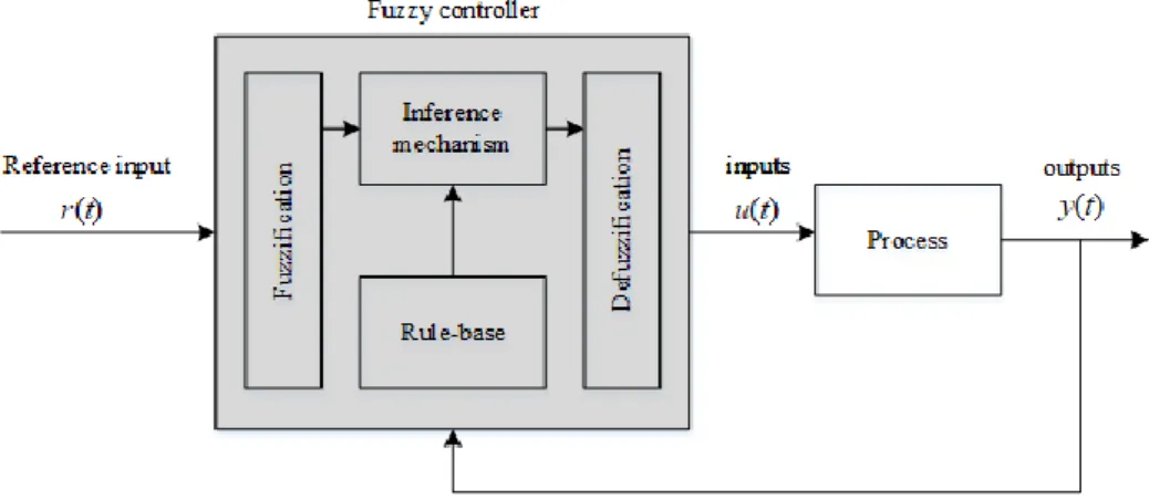
The concept of “Fuzzy sets” was first proposed in 1965 by L. A. Zadeh, an expert in Automatic Control Theory, University of California. Fuzzy control is a kind of control based on fuzzy reasoning and imitating human thinking. It is a kind of control for objects that are difficult to establish accurate mathematical models. The root of its successful application is that fuzzy logic itself provides language information for experts to construct linguistic information and transform it into control strategies. A fuzzy controller is shown in Figure 1-1. The fuzzy controller has several components:
⚫ The rule-base is a set of rules about how to control.
⚫ Fuzzification is the process of transforming the numeric input into a form that can be used by the inference mechanism.
⚫ The inference mechanism uses information about the current inputs (formed by fuzzification), decides which rules apply in the current situation, and forms conclusions about what the plant input should be.
⚫ Defuzzification converts the conclusions reached by the inference mechanism into a numeric input for the plant.
Figure 1-1 Fuzzy control.
8
1.3.3.2 Neural networks
Neural network control is an intelligent control and identification method based on a structure that mimics the physiological structure of the human brain as shown in Figure 1-2.
Figure 1-2 Physiological structure of the neuron.
With the continuous deepening of the application research of artificial neural networks, new models are continuously introduced. In the field of intelligent control, the most widely used are the BP network and the Hopfield network. Compared with the conventional control method the neural network has the following important characteristics:
➢ Non-linearity, the neural network can fully approximate any non-linear function in theory.
➢ Parallel distributed processing, the neural network has a highly parallel structure and parallel implementation capabilities, which makes it have a greater degree of fault tolerance and strong data processing capabilities.
➢ Learning and self-adaptability, neural networks can learn and remember the information provided by the knowledge environment.
➢ Multivariable processing. Neural networks can naturally process multi-input signals and have multi-outputs. It is very suitable for multi-variable systems.
At present, neural networks have been successfully applied in many fields such as signal processing, system identification and optimization, pattern recognition, fault diagnosis and robotics. It will have great and far-reaching significance for the development and application of intelligent control.
9
However, we also see that there are still many problems in the theory and design methods of neural network control for further research, mainly the analysis methods of artificial neural network system stability, the selection and optimization of neural network structure and size, the convergence and real-time problems of learning and control algorithms, and how to apply neural network theory to specific control systems to improve performance, etc.
1.3.3.3 Genetic algorithms
A genetic algorithm (GA) is a computational model that simulates the natural evolution and biological mechanism of Darwin’s biological evolution theory. It is a method to search for the optimal solution by simulating natural evolution of organisms. The main strategy of its operation is to establish the solution set of the population of potential problems of the control object to achieve the encoding of genes. Individuals realize coding, as a combination of multiple genes, from which to start solving a certain gene combination. Just as the adjustment of black hair is a strange thing determined by a certain segment of the chromosome in each subject.
The genetic algorithm also implements the process of mapping phenotype genes to coding and then solving. The main features of the genetic algorithm are:
➢ Take the coding of decision variables as the operation object.
➢ Use the objective function value directly as the search information.
➢ Simultaneous multi-point search of solution space.
➢ Use adaptive probability search technology.
1.3.3.4 Expert control
Expert control developed in the field of artificial intelligence is a technology of knowledge- based intelligent computer programs. The essence of expert control is based on various knowledge of control objects and control laws, and it is necessary to use this knowledge in an intelligent way in order to obtain the optimization and practicality of the control system as much as possible. One simple expert control system is shown in Figure 1-3.
10
Figure 1-3 Expert control.
Expert systems generally consist of a knowledge base, an inference engine, an explanation mechanism, and a knowledge acquisition system. The knowledge base is used to store the empirical knowledge, principle knowledge, feasible operations and rules of experts in a certain field. The original knowledge can be modified and expanded through the knowledge acquisition system. The inference engine solves the current problem according to a certain inference strategy based on the system information and the knowledge in the knowledge base. The interpretation mechanism explains the knowledge found and provides a human-machine interface for the user.
The characteristics of the expert control are as follows:
1) With domain expert-level expertise, capable of symbol processing and heuristic reasoning.
2) Have the ability to acquire knowledge, have flexibility, transparency and interaction.
1.4 Temperature control in industrial process
Temperature control is a common control object in industrial process control and accounts for a considerable proportion of industrial production energy consumption. There many areas where temperature control is required and different industries have different requirements for temperature control. The quality of temperature control directly affects the quality and production efficiency of industrial products. For example, in the beer fermentation process, the proper temperature can greatly increase the speed of beer fermentation and improve production efficiency, the product distillation process requires a higher temperature. Different products
11
may be obtained at different temperatures. The stable temperature can not only speed up the product separation process, but it can also increase the purity of the product. Improving the temperature control of the heating furnace in steel rolling will not only reduce energy consumption, improve production efficiency, but also reduce the occurrence of defective products in steel rolling.
In short, temperature control is one of the most important control objects in industrial processes. Improving the performance of temperature process control is of great significance to industrial production.
The characteristics of temperature control are as follows:
1) Large inertia: Inertia is a property that anything has to maintain its original motion or static state. The inertia of a thing is often related to its quality and its nature. Temperature is a manifestation of the intensity of the molecular motion of an object. It is often because of the slower heat transfer and its larger range of action. It is not easy to change its original temperature, that is, it shows large inertia.
2) Non-linearity: Non-linearity is a situation where the input and output are not proportional.
Temperature and energy are in a linear relationship, but the temperature change is often due to different fuel combustion values, changes in the composition of the heated object or uneven heat dissipation and heating factors, which presents an uncertain characteristic of the relationship between the temperature change and the input given quantity, that is, nonlinear features
3) Large time lag: Because the control of temperature is often not the control of one point of temperature, but the control of the whole thing or a wide range of temperature, the process of temperature rise is often a process from local to overall, so from heating to temperature, the change often takes a certain time, that is, the temperature change has a large lag.
Due to these features of temperature control, coupled with different control objects, difference control accuracy and control requirements, the method of temperature control is also different. The conventional control method is PID control, in order to improve the adaptive range of PID control, fuzzy control and PID control method are combined to generate the fuzzy PID control algorithm. In order to improve the robustness of the controller and the adaptability
12
when the model is changed, a predictive control algorithm can also be introduced. For control objects with coupling effects, decoupling compensation can be applied to reduce the influence between coupling terms. For large time lags. Smith predictive compensation can also be used for control.
In this research, focused on the temperature control system, two main advanced control methods will be proposed: 1) Model-based Pole-Zero cancellation method for the multi-point temperature control system. 2) Model-Free reference model-based artificial neural network control method for the temperature control system with large time lag.
1.5 Main objective
This study will focus on the application of advanced control methods and its application in temperature control systems, and can be mainly divided into two parts: 1) Model-Based Pole- Zero Cancellation Control Method for Multi-point temperature control system. 2) Model-Free Reference-Model-Based Neural Network Method for temperature control system with large lag.
The entire thesis can be divided into four chapters.
Chapter 1: Introduction. In this chapter, a brief overview of the advanced control and its historical development is introduced. The models of the industrial processes and their characteristics are presented. The intelligent control method and the overview of its main areas are introduced. At last, the temperature control system characteristics and difficulties in temperature control are performed.
Chapter 2: The Model-Based Pole-Zero Cancellation method for multi-point temperature control system is introduced including system identification, parameter autotuning, decoupling compensation and pole-zero cancellation control. The presentation flows through theoretical analysis and system simulation to real process experiments. Both simulation and experimental results are finally compared to the conventional PI control system to verify the efficiency of the proposed method.
Chapter 3: The Model-free reference-model-based artificial neural network control method for temperature control system with large time lag is introduced. The systematical introduction of several neural network types is done and the simulations are carried out to evaluate the
13
control efficiency of the proposed method. The experiments are carried out on a DSP based temperature control platform. The results are compared to the conventional I-PD control system to verify the control efficiency of the proposed method.
Chapter 4: The research content of this topic is summarized, and the remaining problems are pointed out, which lays the foundation for further research in the future.
Reference
[1] Lúa. A. Zotică. R C, Skogestad. S, Optimal Operation with Changing Active Constraint Regions using Classical Advanced Control, IFAC-Papers OnLine, 2018, 51, 18, 440-445.
[2] Bagheri. M, Akbari. A, Mirbagheri. S. A, Advanced control of membrane fouling in filtration systems using artificial intelligence and machine learning techniques: A critical review, Process Safety and Environmental Protection, 2019, 123, 229-252,
[3] Jin. S, Zhao. B. T, Su. Y. X, Advanced control of NO emission from algal biomass combustion using loaded iron-based additives, Energy, 2019, 185, 229-238.
[4] Tahir. F, Mercer. E, Lowdon. I, Lovett. D, Advanced process control and monitoring of a continuous flow micro-reactor, Control Engineering Practice, 2018, 77, 225-234.
[5] Shao. G. D, Latif. H, Villalba. C. M, Denno. P, Standards-based integration of advanced process control and optimization, Journal of Industrial Information Integration, 2019, 13, 1-12.
[6] Zhou. Y, Lorenz T, Advanced-step multistage nonlinear model predictive control: Robustness and stability, Journal of Process Control, 2020, 85, 15-29.
[7] Choi. J. S, Kim. K. M, Changes in infection control policies and advancing infection control advanced practice nurse education in the Republic of Korea, American Journal of Infection Control, 2019.
[8] Zhou. J, Lorenz T, Advanced-step multistage nonlinear model predictive control: Robustness and stability, Journal of Process Control, 2019, 84, 192-206.
[9] Manoli. K, Sarathy. S, Maffettone. R, Domenico Santoro, Detailed modeling and advanced control for chemical disinfection of secondary effluent wastewater by peracetic acid, Water Research, 2019, 153, 251-262.
[10] Zhou. P, Lu. S, Yuan. M, Chai. T, Survey on higher-level advanced control for grinding circuits operation, Powder Technology, 2016, 288, 324-338.
14
[11] Sangi. R, Müller. D, A novel hybrid agent-based model predictive control for advanced building energy systems, Energy Conversion and Management, 2018, 178, 415-427.
[12] Lv. Y, Qian. S, Du. S, Chen. J, Zhou. J, Xu. C, Coupling feedback genetic circuits with growth phenotype for dynamic population control and intelligent bioproduction, Metabolic Engineering, 2019, 54, 109-116.
[13] Joyce. P, Gustafsson. H, Engineering intelligent particle-lipid composites that control lipase-mediated digestion, Advances in Colloid and Interface Science, 2018, 260, 1-23.
[14] Morillo. D, Olaby. O, Granero. M. A, Physiological closed-loop control in intelligent oxygen therapy:
A review, Computer Methods and Programs in Biomedicine, 2017, 146, 101-108.
[15] Khayyam. H, Ranjbarzadeh. H, Marano. V, Intelligent control of vehicle to grid power, Journal of Power Sources, 2012, 201, 1-9.
[16] Zhang. L, Zhou. L, Ren. L, Lai. L, Modeling and simulation in intelligent manufacturing”, Computers in Industry, 2019, 112, 103-123.
[17] Ma. H, Yu. C, Dong. L, Fu. Y, Shuai. C, Sun. H, Zhu. X, Review of intelligent well technology, Petroleum, 2019.
[18] Magdi. S, Nezar. M, Mohamed. I, Adaptive intelligent techniques for microgrid control systems: A survey, International Journal of Electrical Power & Energy Systems, 2017, 90, 292-305.
[19] Dai. Y, Zhu. Z, Shan. Z, Cheng. Z, A Survey on Intelligent Screening for Diabetic Retinopathy, Chinese Medical Sciences Journal, 2019, 34, 2, 120-132.
[20] Cao. H, Zhang. X, Chen. X, The concept and progress of intelligent spindles: A review, International Journal of Machine Tools and Manufacture, 2017, 112, 21-52.
[21] Alessa. D, Jason. DM, Micro needling Options for Skin Rejuvenation, Including Non–temperature- controlled Fractional Microneedle Radiofrequency Treatments, Facial Plastic Surgery Clinics of North America, 2020, 28, 1, 1-7.
[22] Petrie. M. D, Wildeman. A. M, Bradford. J. B, Hubbard. R. M, A review of precipitation and temperature control on seedling emergence and establishment for ponderosa and lodgepole pine forest regeneration, Forest Ecology and Management, 2016, 361, 328-338.
[23] Zhou. J. K, Claridge. D. E, PI tuning and robustness analysis for air handler discharge air temperature control, Energy and Buildings, 2012, 44, 1-6.
15
[24] Xu. X, Zhong. X, Deng. S, Zhang. X, A review on temperature and humidity control methods focusing on air-conditioning equipment and control algorithms applied in small-to-medium-sized buildings, Energy and Buildings, 2018, 162, 163-176.
[25] Michael. J. F, Myron. P. Z, Climate change and biological control: the consequences of increasing temperatures on host–parasitoid interactions, Current Opinion in Insect Science, 2017, 20, 39-44.
[26] Zhang. T, Liu. X, Jiang. Y, Development of temperature and humidity independent control (THIC) air-conditioning systems in China—A review, Renewable and Sustainable Energy Reviews, 2014, 29, 793-803.
[27] Bakir. T, Bonnard. B, Rouot. R, Geometric optimal control techniques to optimize the production of chemical reactors using temperature control, Annual Reviews in Control, 2019, 48, 178-192.
[28] Shaterabadi. Z, Nabiyouni. Z, Soleymani. M, Physics responsible for heating efficiency and self- controlled temperature rise of magnetic nanoparticles in magnetic hyperthermia therapy, Progress in Biophysics and Molecular Biology, 2018, 133, 9-19.
[29] Sevil. Ç, Zehra. Z, Hale. H, Mustafa. A, Optimal temperature control in a batch polymerization reactor using fuzzy-relational models-dynamics matrix control, Computers & Chemical Engineering, 2006, 30, 9, 1315-1323.
[30] Michael. W, Temperature Control of Premature Infants in the Delivery Room, Clinics in Perinatology, 2006, 33, 1, 43-53.
16
Chapter 2
Pole-Zero Cancellation Method for MIMO Temperature Control System
2.1 Experimental setup
Before the control method is designed and applied, the experimental setup needs to be introduced first. The designed method will be applied to the experimental setup shown in Figure 2-1. It includes a digital signal processor (DSP) as the temperature controller. The system has four coupled channels. Each channel has two independent heaters and one temperature sensor.
The temperature sensor transforms the temperature (0-400degree Celsius) into an output voltage (0-10VDC). The heaters are controlled by the solid-state relay (SSR has shown in Figure 2-1), and the SSR is driven by pulse width modulation (PWM) signals. The temperature can be controlled through the duty ratio of the PWM signals.
(a) Front view (b) Rear view
Figure 2-1 Experimental setup.
2.2 System identification
In order to realize precise temperature control by the model-based advanced control method, the mathematical model of the control object needs to be obtained, thus, the system identification needs to be carried out.
17
2.2.1 System identification methods
System identification is based on the input and output time functions of the system to determine the mathematical model describing the behavior of the system. It is a branch of modern control theory. The main problem of analyzing the system is to determine the output signal according to the input time function and the characteristics of the system. The conventional system identification methods can be divided into three categories:
1). Step response method: This method generally refers to the output (response) of the system when the input is a step function in units.
2). The least-squares (LS) method: This method is a conventional data processing method.
But because the least-squares estimation is non-uniform and biased, so in order to overcome its shortcomings, there have formed a number of identification methods based on the least-squares method.
3). Maximum likelihood method: The maximum likelihood method (ML) has very good performance for special noise models, and has good theoretical guarantees. But the calculation cost is large, and may get the local minimum of the loss function.
2.2.2 Step response system identification method
For our control object, the temperature system is a non-linear and time-continuous system, thus, the step response system identification method has been introduced. The theoretical of the step response identification is performed as follows.
In general, the numerator and denominator of the transfer function of a closed-loop system are polynomial of s, which can be written as Eq. (2-1)
( ) ( ) ( )
1
1 1 0
1
1 1 0
m m
m m
n n
n n
C s b s b s b s b
s R s a s a s a s a
− −−
−
+ + + +
= =
+ + + + (2-1)
The Eq. (2-1) can be expressed as the product of the following factors as Eq. (2-2).
18
( ) ( ) ( )
( )
( )
1
1 m
i i
n
i i
K s z
s C s
R s s s
=
=
−
= =
−
(2-2)In practical control systems, all closed-loop poles are usually different. Therefore, when the input is a unit step function, the output can be expressed as Eq. (2-3)
( ) ( )
( ) ( )
1
2 2
1 1
1 2
m i i
q r
j k k k
j k
K s z
C s s
s s s s
=
= =
−
=
− + +
(2-3)Where q and r satisfy the relationship as shown in Eq. (2-4).
2
q+ r=n (2-4)
In the equation, q is the number of real poles, r is the logarithm of conjugate complex poles.
Assuming that 0<ζ<1, extend Eq. (2-3) into the partial fractions as Eq. (2-5):
( )
0 2 21 1 2
q r
j k k
j j k k k k
A A B s C
C s s = s s = s s
= + + +
− + +
(2-5)Assuming that all initial conditions are zero, inverse Laplace transform of Eq. (2-5) can be used to obtain the unit step response of higher-order systems as shown in Eq. (2-6).
( )
0 - 21 1
- 2
1 2
e e cos( 1 ) +
e sin( 1 ) , 0
1
j k k
k k
q r
s t t
j k k k
j k
r
k k k k t
k k
k k k
h t A A B t
C B
t t
= =
=
= + + −
− −
−
(2-6)From Eq. (2-6), the time response of the higher-order system is composed of the time response function terms of the first-order system and the second-order system. At the same time, Eq. (2-1) can be written as Eq. (2-7).
19
( ) ( ) ( )
( ) ( )
1
1 1 0
1
1 1 0
1
1 1 0
2 2
1 1
1 2
2 2
1 1
2
2 2
1 1
2
2
1 2
, 2
m m
m m
n n
n n
m m
m m
q r
i j nj nj
i j
q r
i j
i i k j nj nj
n m
n j j i
i i j j j j
B s b s b s b s b
G s A s a s a s a s a
b s b s b s b
s p s s
k k
s p s s
K K
T s s s
m n q r n
−
− −
−
−
−
= =
= =
+
= =
+ + + +
= =
+ + + +
+ + + +
=
+ + +
= +
+ + +
= +
+ + +
+ =
(2-7)
According to this equation, a high order system can be decomposed into Figure 2-2.
Figure 2-2 Decomposition of higher-order linear system model.
To sum up, an estimation model of a higher-order system can be obtained by paralleling several first-order and second-order typical links, and the step response of the parallel model is used to approximate the step response of the actual system, thereby obtaining the mathematical model of the actual system.
Furthermore, the third-order and lower-order estimation models are combined through first- order and second-order typical links and the shape of the decomposition curve of the system model is adjusted by adjusting parameters to continuously approximate the step response of the higher-order system. The step response of the original high-order system is small compared to the error. Depending to the input and output characteristics, it can reflect the overall
20
characteristics of the original system. So that the third-order and lower-order systems can be used to equivalent high-order systems to find the transfer function.
2.2.3 Time domain analysis of linear systems
The evaluation of control system performance is divided into dynamic performance indicators and steady-state performance indicators. The dynamic performance indicators can reflect the response speed and damping range of the system, while steady-state performance indicators can reflect the control accuracy and anti-disturbance ability of the system. In practical applications, the commonly used dynamic performance indicators are mostly rising time tr, which is a measure of the response speed of the system, overshoot δ% that evaluates the degree of damping of the system. The adjustment time ts is a comprehensive index that reflects both the response speed and degree of damping.
2.2.3.1 First-order systems
A typical first-order system can be expressed as Eq. (2-8).
( )= 1
G s K
Ts+ (2-8)
The steady-state gain K determines the steady-state response value, and the time constant T determines the step response speed. The larger T is, the slower the response and the longer the rising time.
2.2.3.2 Identification method for first-order system
From Eq. (2-8), the system identification algorithm for the first-order system is as follows:
1) Steady-state gain K
( ) ( )
0K=y −y (2-9)
In this equation, y(∞) represent the steady-state value of the step response and y(0) represents the initial value.
21
2) Time constant T
Next, we need to find the coordinate point on the step response curve when the output changes to 95% of the final value. Its corresponding time is the adjustment time, which according to the dynamic performance index of the first-order system, it is known that ts is three times of T, thus time constant T can be obtained as:
3 ts
T = (2-10)
2.2.3.3 Verification of identification accuracy
In order to verify the identification method of the first-order system, the simulation has been carried out. Assuming that the identified system transfer function is as Eq. (2-11):
( ) 5
100 1
P s = s
+ (2-11)
A step signal is applied at the initial moment of the simulation, the simulation result is shown in Figure 2-3 and the identified system transfer function is as Eq. (2-12), the fitness is defined as the squared error between the system response and the identified system response.
Figure 2-3 Identification result of first-order system.
( ) 5
99.973 1
P s = s
+ (2-12)
22
2.2.4 System identification of first-order plus time delay
2.2.4.1 Identification algorithm
In the temperature control system, the dead time is very large and can’t be ignored, thus the above identification method needs to be improved. The typical identification structure of a linear plus delay time system is shown in Figure 2-4.
Figure 2-4 Typical identification structure of open-loop plant.
A linear single input single output system with pure delay time can be described as follows:
( )n
( )
( )m( ) ( )
n m
a y t =b u t− +e t (2-13)
, 1 0
1(n 1)n n n
a = a a− a R + (2-14)
, 1 0
1(m 1)m m m
b = b b − b R + (2-15)
( )n
( )
( )n( )
, ( )n 1( )
( )0( )
1( )n 1y t =y t y − t y t R + (2-16)
( )m
( )
( )m( )
, (m 1)( )
( )0( )
1(m 1)u t− =u t− u − t− u t− R + (2-17)
Where, y(i) and u(i) respectively indicate the ith order differentials of y and u, e(t) is the error term. Perform the Laplace transform at both sides of the above equation, the Eq. (2-18) can be obtained.
( ) ( )
e + 1 1( )
n m s n
n m n
a s Y s =b s U s − c s− − +E s (2-18)
Y(s), U(s) and E(s) are the Laplace transform of y(t), u(t) and e(t), respectively. And at the same time the following equation can also be obtained as is shown in Eq. (2-19):
( ) ( )
e + 1 1( )
n m s n
n m n
a s Y s =b s U s − c s− − +E s (2-19)
The element cn-1 captures the initial conditions and is defined as:
11 1, 2 0 n
n n n
c− = c − c− c R (2-20)
23 (n 1)
( )
0 , 1n i i
c− =h y − i= n (2-21)
( )
1 1
(i 1)
0 n i n
i n n
h = − a a − − R (2-22)
( )n 1
( )
0 ( )n 1( )
0 , (n 2)( )
0( )
0 Ty − = y − y − y (2-23)
A filter with dynamic integration and order lag term is introduced to form an iterative algorithm to estimate model parameters and pure lag time simultaneously. The filter used in this paper has the following form of transfer function as shown in Eq. (2-24):
( )
1( )
P s =sA s (2-24)
Among them, A(s) is the denominator of the process transfer function. The function of the integration link is to decouple the pure lag from the dynamic parameters of the model. The function of the 1/A(s) term is to avoid the direct differential effect of the noise signal. Add the filtering terms P(s) on both sides of Eq. (2-24), and get the formula as Eq. (2-25).
( ) ( ) ( ) ( )
e + 1 1( ) ( ) ( )
n m s n
n m n
a s P s Y s =b s P s U s − c s− −P s +E s P s (2-25)
Using partial fraction expansion, the filter's transfer function can be expanded as follows:
( ) ( ) ( )
1 C s 1
sA s = A s +s (2-26)
Among them, 𝐶(𝑠) = −(𝑎𝑛𝑠𝑛−1+ 𝑎𝑛−1𝑠𝑛−2+ ⋯ 𝑎1), defining that 𝑌𝐼(𝑠) = 𝑌(𝑠)/𝐴(𝑠) , 𝑌(𝑠) = 𝑌(𝑠)/𝐴(𝑠), use the same notation for U(s) to transform the estimated equations into standard least squares form:
( )
1( )
1( )
e 0( ) ( ) ( )
e 1 1( ) ( )
I n m s I s n
n m n
Y s = −a s Y s− +b s U s− − +b C s U s +U s − +c s P s− − + s (2-27) Where an is an removes the last item, bmis bm removes the last item, and bmR1m
For the step input, if the step amplitude is h, that is u(t) = ur(t) – uss = h, we can obtain Eqs.
(2-28) and (2-29), respectively:
( )
hU s = s (2-28)
( ) ( )
( ) ( ) ( )
U s h
U s hP s
A s sA s
= = = (2-29)