How customer satisfaction affects loyalty:
Insights from nonlinear hierarchical Bayes
modeling of customer satisfaction index
著者
Xing Aijing, Terui Nobuhiko, Kannan P.K.
journal or
publication title
TMARG Discussion Papers
number
124
page range
1-37
year
2016-04
TOHOKU MANAGEMENT
&ACCOUNTING RESEARCH GROUP
Discussion Paper No. 124
How customer satisfaction affects loyalty:
Insights from nonlinear hierarchical Bayes modeling
of customer satisfaction index
Xing Aijing, Nobuhiko Terui and P.K.Kannan
April 2016
GRADUATE SCHOOL OF ECONOMICS AND MANAGEMENT TOHOKU UNIVERSITY KAWAUCHI, AOBA-KU, SENDAI 980-8576 JAPAN
1
How customer satisfaction affects loyalty:
Insights from nonlinear hierarchical Bayes modeling of customer satisfaction index
Xing Aijing, Nobuhiko Terui1 and P. K. Kannan Tohoku University and University of Maryland
April, 2016
Abstract
The paper investigates the nonlinear relationship between customer satisfaction and loyalty. We extend the relationship proposed by the customer satisfaction index (CSI) model to include a nonlinear functional form between satisfaction and loyalty. We examine different functional forms on how satisfaction affects loyalty and propose a model that reflects intrinsic
characteristics of nonlinear effects, such as saturation-attainable limit of effectiveness, non-constant marginal return, and asymmetric response between satisfied and dissatisfied customers, in a parsimonious way. The model is estimated via a hierarchical Bayes model to accommodate structural heterogeneity of companies surveyed in the analysis. The key contributions of the paper include a nonlinear structural equation model that includes nonlinear term of endogenous latent variable and an efficient algorithm of MCMC in terms of multi-move sampler by using Gibbs sampling.
The empirical analysis by using survey data shows that (1) hierarchical Bayes models estimated by borrowing other companys’ data are better than the independent model using their own data in terms of not only goodness of fit measures but also in the number of significant model estimates, (2) nonlinear models perform better than linear models, (3) nonlinear model with asymmetric marginal returns and attainable limits is found to be the best model. The managerial implications for loyalty management include: (i) there are limits to attainable levels of loyalty through satisfaction; (ii) the phenomenon of loss aversion is observed in customers’ responses; (iii) marginal return of satisfaction is asymmetric across satisfied and dissatisfied customers, i.e., increasing for dissatisfied customers and decreasing for satisfied customers, (iv) in general, direct effect of satisfaction is more significant than indirect effect through recommendation intention.
Finally, based on the estimated response curve of loyalty as a function of satisfaction and the empirical distribution of customers on the dimensions of CSI scores, we evaluate the efficiency of loyalty programs under assumptions of full and limited access to customers.
2
1. Introduction
The relationship between customer satisfaction and loyalty has been one of the widely studied relationships in marketing and services literature (Dong et al 2011; Kumar et al 2013). The premise that customer satisfaction, a construct that underlies customers’ perceptions regarding their overall consumption experiences (Anderson and Salisbury 2003), significantly impacts customer loyalty, a construct that drives customer retention and repurchase behavior, is key to firms’ customer orientation. It is this this relationship that forms the basis for measuring marketing effectiveness (Fornell 1992, Bolton and Lemon 1999, Anderson et al. 2004), and for firms’ market and financial performance and for firm value (Anderson and Mittal 2000; Gupta, Lehmann and Stuart 2004, Gupta and Zeithaml 2006). The fact that this relationship has been extensively studied in marketing and services over several decades highlights its important and critical role in determining the effectiveness of marketing programs and ensuring the creating of firm value through marketing action.
In this paper, we examine the relationship between customer satisfaction and customer loyalty by using the survey data used for developing customer satisfaction index. The framework of analysis uses the customer satisfaction index (CSI) model as the starting point to propose a nonlinear structural equation model which includes a nonlinear function form between satisfaction and loyalty as one equation in the set of equations. We contribute to the existing literature that examines satisfaction and loyalty variables which are measured by comprehensive system of equations (Dong et al 2011; Kumar et al 2014), in contrast to previous studies using just the metrics of satisfaction in isolation of their context.
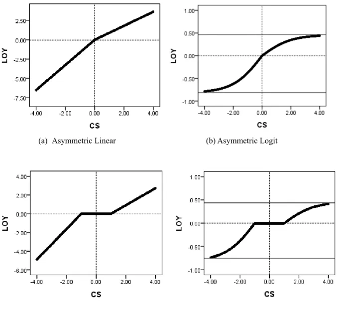
As for functional forms of the nonlinear relationship, we consider piecewise linear and S-shaped functions. The former is motivated by the ease of estimation, being close to linear model and the latter specification is justified by prospect theory of Kahneman and Tversky (1979) and empirically supported by Ngobo (1999), whose research objective and dependent variable of loyalty are common with ours.
From the methodological point of view, there are quite a few extant papers on nonlinear structural equation models, for example, Lee (2007) discusses a model with nonlinearity only with respect to exogenous latent variables. This article contributes to the modeling literature by the modeling nonlinear structural equations that include nonlinear terms of endogenous latent variable. By using the recursive property of system for CSI model, implying that latent variables are determined sequentially, we provide an efficient algorithm of MCMC in terms of
3
multi-move sampler for latent variables by using Gibbs sampling.
In addition, we employ a hierarchical Bayes model to deal with structural heterogeneity across individual companies in the survey data. The model connects the structural models for respective company, and it leads to higher reliability of model estimates than the original customer satisfaction index model. This is accomplished by using the insights from Terui et al. (2011).
Section 2 discusses extant work on nonlinear relationship between satisfaction and outcomes including loyalty in the literature. We also discuss the perspective for building the framework of our analysis. In section 3, we propose the model, including possible alternative
specifications. Section 4 reports the empirical results of model comparison, parameter estimates, the interpretation of estimates and derived managerial implications. Section 5 presents the conclusions.
2. Nonlinear Relationship between Customer Satisfaction and Loyalty 2.1. Nonlinear Relations of Satisfaction
There are many extant works on nonlinear relationships between satisfaction and outcome variables. They investigate customer satisfaction relationship with one of firm’s outcomes by using different metrics. Most of the studies show that satisfaction has a positive and nonlinear asymmetric impact on firm’s outcomes, and different functional forms are supported by these studies (Dong et al 2011, Kumar et al 2014).
Fornell (1992) empirically showed that the relationship between customer satisfaction and their intention to repurchase goods or services is nonlinear, and dissatisfaction has greater influence than satisfaction on customers’ repurchase intentions. Mittal and Kamakura (2001) examined levels of customer satisfaction and dissatisfaction impacting purchase intention and actual purchase behavior. They found that linear methods may underestimate the influence of satisfaction and suggest nonlinear relations whose patterns are moderated by consumer
heterogeneity across the attributes. Keiningham et al (2003), Bowman and Narayandas (2004), and Cooil et al. (2007) showed that the satisfaction affects the share of wallet nonlinearly. Homburg, Koschate and Hoyer (2005) suggest inverse-S shaped for willingness to pay by using experimental study. On the other hand, Ngobo (1999) examined the relation between
4
function for the relationship.
2.2 Nonlinearity and Moderating Effects
Nonlinearity has been investigated in the context of moderating effects on the relationship between satisfaction and outcome variables. In particular, Jones and Sasser (1995) clarified that the competitive environment of the market affects the nonlinear relationship between satisfaction and loyalty. Their empirical research involved more than 30 companies in five industries (local telephone companies, airlines, hospitals, personal computers, and
automobiles) and showed that the competitive environment greatly influences the relationship between customer satisfaction and loyalty.
Bloemer and Ruyter (1998) demonstrated nonlinearity by incorporating involvement as the key parameter between customer satisfaction and loyalty. Based on customers expressing equal levels of satisfaction, their comparative study showed that highly involved customers exhibit greater loyalty than customers with low involvement. Mittal and Kamakura (2001) and Cooil et al. (2007) discuss nonlinearity in the context of the moderating effect of consumer characteristics. Recently, Eisenbeiss, Corneliben, Backhaus and Hoyer (2014) investigate nonlinear and asymmetric return on satisfaction to willingness-to-pay by considering two kinds of moderating effects – firm reputation and consumer’s involvement.
2.3 Framework of Our Study
In most prior research, satisfaction and loyalty variables are directly measured by using a survey directed to respondents. The impact of other antecedents on satisfaction is also not taken into consideration. On the other hand, Fornell (1992) discusses the need to use a comprehensive system of post-purchase outcomes in the way that satisfaction is part of the overall outcome that is measured. This is motivated by the fundamental principles that a variable should take on meaning depending on the context (Fornell, 1982, 1988; Fornell and Yi, 1992), survey variables contain some degrees of errors (Andrews, 1984), and satisfaction is not directly observable (Howard and Sheth, 1969, Oliver, 1981, Westbrook and Riley, 1983). In addition, he insists that, if satisfaction variable is measured in isolation of the context and it is used retrospectively to estimate the relationship, we tend to have the results with low reliability and strongly biased parameter estimates.
5
loyalty as latent variables, i.e., customer satisfaction index (CSI) model by Fornell, et al. (1996). However, CSI model premises a linear relationship between latent variables, and we extend the model to propose a nonlinear structural equation model which includes nonlinear function from satisfaction to loyalty.
3. Nonlinear CSI Model
3.1 Customer Satisfaction Index Model
The customer satisfaction index uses the only uniform measure of customer satisfaction that allows comparison between companies and bench-marking across industries. It also illustrates how customer satisfaction is embedded in a system of cause–effect relationships. Furthermore, this index is significant as a leading indicator of the financial results of the company (Anderson et al., 2004; Fornell et al., 1996, 2010). They employ the adopted expectancy disconfirmation as a basic theory which was proposed by Oliver (1980). It is a model in which the level of customer satisfaction is decided by the degree of disconfirmation between perceived quality after a purchase and customer expectation before a purchase.
The CSI model describes that customer expectations drive perceived quality and perceived value, and these three latent variables generate customer satisfaction. Customer satisfaction in turn directly affects customers’ voice and loyalty. The model estimation employs 17 manifest variables, which are ordered categorical variables based on survey questions rated on a scale of 1–10 (low–high). The scores of customer satisfaction are factor scores for n sampled
customers’ satisfaction, and they are reported as standardized metrics between 0 and 100 points. Full description of model is provided in Appendix A. Using identical structure model for companies allows us to compare satisfaction level between companies, and the changes in it over years.
3.2. Nonlinear Model on the Satisfaction to Loyalty
Customer loyalty (LOY) is a function of customer satisfaction (CS) and recommendation to others (RE) (“Voice” in original CSI) and the model is described as one equation in the set of equations of CSI model by
i i i i
LOY
CS
RE
(1) where i means the index for respondent (customer),
iis the normally distributed error term,6
and
,
are path coefficients.The linear specification is reasonable as local approximation to possibly more complicated relations, but it has limitations in failing to accommodate some characteristics discussed in the literature, i.e., (i) not constant return to scale, (ii) saturation effects and (iii) asymmetric response. These are well captured by nonlinear models.
We model the accommodation of these characteristics in a parsimonious way as follows:
( )1
1
( )1
1
1
1 exp
2
1 exp
2
i i i i iLOY
I
I
RE
CS
CS
(2)where I is the indicator function taking 1 if
CS
i
0
and zero otherwise. The shape of function is depicted in Figure 1. This function is in line with Prospect Theory (Kahamenan and Tversky, 1979) and empirically supported by Ngobo (1999) whose research objective and dependent variable of loyalty closely resemble ours in the literature.Figure 1: Nonlinear Model for Satisfaction to Loyalty
This function captures nonlinear effects in terms of logistic function. That is, it has asymmetric response around the inflection point, i.e.,
CS
0
, which is fixed foridentification of model, and also the marginal return to LOY is changing at every level of CS. The upper limit represents the satiation level and the lower limit indicates the baseline independent of CS. They are respectively provided by
1
( )2
and
1
( )2
. Thus the estimates of coefficients
( ) and
( ) determine the maximum and minimum levels ofloyalty caused by satisfaction. They also define the speed to reach these limits in respective regimes. They provide several interesting implications for service management. The company with larger
( ) value will attain the attainable limit of loyalty quickly byadditional effort on satisfaction as long as it stays in the positive regime. On the other hand, the smaller value of
( ) shows that the increasing rate of return is slower although the7
model suggests that, given a level of CS score, companies obtain useful information on how additional effort on the customer satisfaction dimension impacts the relative to the speed of return to CS increases and the attainable limit to loyalty. We call model (2) as “asymmetric logit model.”
When we replace the logistic function by simply
CS
i as a piece-wise linear term, we obtain the “asymmetric linear model” which we use for comparison purposes in the empirical application.
( ) ( )
1
i i i i i
LOY
I CS
I
CS
RE
(3) This model defines different slopes of linear response in respective regimes. It approximates nonlinear relation by piecewise linear functions, and it does not have attainable limits since it models the relationship locally, even though it has more useful information than a simple linear model. In addition, we consider the inverse S-shaped models, as is discussed in Homburg et al. (2005), by introducing thresholds,r
1 andr
2, in the satisfaction domain, which define thezone of tolerance.
1 2 ( , )r ( , )r 1 i i i i i LOY
I CS
I CS
RE
(4)where
( , )r1 takes some value when1
0
iCS
r
and zero otherwise,
( , )r2 takes some value when0
r
2CS
i and zero otherwise. We call this “threshold linear model”. Similarly, “threshold logit model” is specified as
1 2 ( , )1
1
( , )1
1
1
1 exp
2
1 exp
2
r r i i i i iLOY
I
I
RE
CS
CS
(5)We compare these alternative models in the empirical application. The functions of these models are depicted in Figure 1 for comparison.
We employ these nonlinear models just for the customer satisfaction to loyalty relationship nd keep linear structural equations for other relations in CSI model. Full description of our model is given at Appendix A.
8
3.2. Hierarchical Bayes Modeling for Stable Estimation
The CSI model assumes that every company has the identical structure on customer satisfaction for the purpose of comparing the services across different companies, and thus is aggregated to industry groups and national levels. However, each company should have structural heterogeneity on customer satisfaction measures. The structural heterogeneity appears to produce the result that some path coefficient estimates are not significant for some companies, which leads to reduce the credibility of scores. To overcome this problem, Terui et al. (2011) proposed the hierarchical Bayes modeling of customer satisfaction index to increase reliability of model estimates not only on the goodness of fit, but also by the number of significant estimates of path coefficient. That is, HB model produces larger number of
significant estimates in the model and better goodness of fit than independently estimated model. This result comes from the property that HB modeling borrows information of neighbors by pooling data to get the stable estimate of parameters on the assumption that they share homogeneity in some aspects regardless of independent information.
In this study, we employ HB modeling which relates the model of each company 1,..., h H such that
' ; , h h h h Nk V β Θ z η η 0 , (6) whereβ
h is the vector of path coefficients between latent variables andz
h is attribute data for the company h, andη
his error term. This is prior distribution on the path coefficientsh
β
, and this means that the path coefficients are not independent and restricted by the commonparameter (
Θ
,V
). The prior specification (6), together with appropriate prior specifications9
likelihood based to constitute joint posterior density,
h , hi , , | Data
p β ω ΘV . (7)
The numerical evaluation of this density is conducted by Markov chain Monte Carlo (MCMC), and its algorithm is described together with prior specifications in Appendix B.
4. Empirical Results 4.1. Data
The dataset is available from the Japanese CSI development working group managed by the Japanese Agency of Service Productivity and Innovation Growth. We use the data for survey conducted in 2008 year, and it includes 21 companies in three industries—mobile
telecommunications (4), convenience stores (5), hotels (12). The sample sizes used in analysis are: mobile telecommunications (company1 = 456, company2 = 456, company3 = 360),
convenience stores (company1 =456, company2 = 456, company3 = 360), hotels (company1 = 300, company2 = 300, company3 = 300).
4.2. Data Transformation and Full Conditional Posterior Density for Estimation
We employ Bayesian inference on the model estimation as is explained in Lee (2007) and Terui et al.(2011) on the grounds of distributional property of observations as well as derived
distribution of estimated satisfaction scores. The data are measured by 10 point Likert scale. Thus the ordered categorical data are not consistent with normality assumption. On the other hand, the structural equation model is developed on the assumption of normality on variables. The American CSI model employs PLS method for model estimation since PLS does not
assume any distribution on the error terms to estimate the model parameters. However, there is no free lunch. In fact, Terui et al. (2011) compares the estimates by Bayesian MCMC method with those by PLS, and it demonstrated that the distribution of estimated satisfaction score by PLS method is mostly skewed, on the other hand, the score distribution evaluated by Bayesian MCMC algorithm is stable and symmetric. The satisfaction score is calculated by taking sample mean of estimated respondent’s scores, and being standardized to be inside 0 and 100 points, and the satisfaction score must be reasonable only when the distribution is symmetrical.
10
data into continuous variable, which follows the specified normal distribution by way of data augmentation (Lee, 2007; Terui et al., 2011). We introduce a set of cut points across the normal distribution to decompose it into 10 segments that may be categorized on a scale of 1 to 10. Thus, the probability of each region corresponds to the probability mass of each ordered category. When we have a categorical sample, we generate the samples from the truncated normal distribution whose cut points are defined by the corresponding segment.
The algorithm for Bayesian inference of linear structural equation model is given by Lee (2007). By using the special properties of CSI model that the latent variables
, , , , ,1 2 3 4 5
'
are determined sequentially by the initial driving force of “expectation
”, in the way that
1
2
3
4
5 and also the nonlinear equation of
5(LOY)by
3(CS) is positioned in the last. The efficient algorithm is available for generating posterior distribution of latent variables. We first decompose the set of latent variables into linear and nonlinear parts
1
, , , ,1 2 3 4
' and
5. Then we express the joint prior density is defined by p
p
1 p
5| 1
to derive marginal posterior density of linear latent variables
1 and conditional density of nonlinear latent variable of
5on
1 (i)
[ 1]
1| , 1 | , p
x
p
p x
(ii)
[ 5]
5 | 1, , 5 | 1 | , p
x
p
p x
where
means the set of model parameters including factor loadings, path coefficients, and variances, and x is data. The algorithm for linear part (i) is given by Lee (2007). The nonlinear part (ii) is the product of normal prior and normal likelihood, and thus the posterior density is analytically derived by using conjugate property. That is, multi-move sampler is available for latent variables of our model. The path coefficient parameters are defined as linear in our model, and the algorithm for linear structural equation model is available, together11
with other parameters of factor loadings and variance, in Lee (2007). The details are explained in the algorithm section in Appendix B.
Finally, the conditional posterior density of model parameter,p
| ,x
, is available inLee (2007) since this is the same structure conditional on latent variables with linear structural equation model. The details of full conditional posterior density are provided in Appendix B. 4.3. Model Comparison
We estimated the parameter using Markov chain Monte Carlo (MCMC) by the use of Gibbs sampling. This section reports results of the comparison between models by comparing the values of Deviance Information Criterion (DIC), an information criterion of Bayesian analysis as well as log of marginal likelihood (LML).
We compare (i) linear model, (ii) logit model, (iii) asymmetric linear model, and (iv) asymmetric logit model in their HB estimations. As a benchmark model, we also set the original CSI model, denoted by (0) independent linear model.
Table 1:Model Comparison: DIC and log of Marginal Likelihood
Table 1 shows the calculated values of DIC and LML for the different models. First of all, both measures support the HB models than independent linear model, and the advantage of HB modeling is more evident for the measure of LML. The comparison between linear and nonlinear models supports nonlinear models by both criteria, and within groups, asymmetric response models are supported more than symmetric models: HB asymmetric linear model is better than HB linear model, and HB asymmetric logit model performs better than HB logit model in case of DIC. We note that LML of HB logit model slightly shows better fit than HB asymmetric logit model. However, the latter model contains double number of response parameter as the former, and we employ DIC which discounts the number of parameter more appropriately than LML.
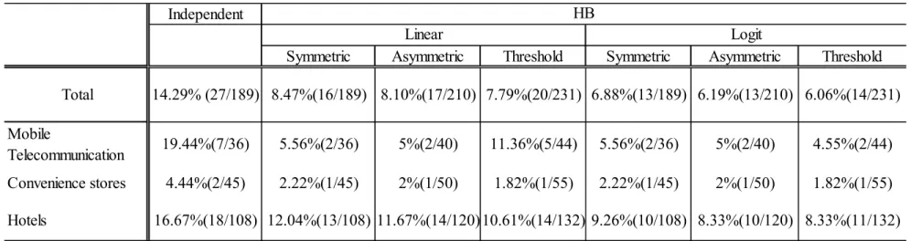
Table 2 tabulates the number of path coefficients that were not significant in the sense of 95% highest probability density (HPD) region for respective models. The total number of insignificant estimates in each model is shown at the bottom of table. The effect of HB modeling that borrows other company’s data on the estimates is evident. The number of
12
insignificant estimates in (0) independent model is drastically reduced from 27 to 16 for (i) HB linear; 17 for (ii) HB asymmetric linear; 13 for (iii), (iv) HB (asymmetric) logit models. The heterogeneity in industry is evident to see that hotels have relatively more insignificant estimates.
Table 2: The Effect of HB modeling on Estimate of Path Coefficients
The examination of results on model fit criteria in Table 1 and the number of significant parameters estimate in Table 2 shows the order of better model is HB asymmetric logit, HB logit, HB asymmetric linear, and HB linear models. The asymmetric response is better supported and furthermore the model gets more advantageous if the saturation effects are incorporated in the model.
4.4. Parameter Estimates of Nonlinear Term from CS to LOY
Table 3.1 shows the estimates (posterior mean) of coefficient of
( ) and
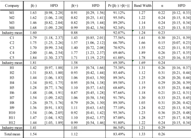
( ) of nonlinear term from satisfaction to loyalty for individual companies. 95% HPD region is also given next to the estimate. The industry level estimates given in Table 3.2 are derived from posterior means of industrial dummy in the hierarchical model.Table 3.1: Parameter Estimates (Company Level) Table 3.2: Parameter Estimates (Industry Level)
First of all, path coefficients are significant for all companies as HDP region does not include zero with the level of 95% probability. Second, we observe the estimate of
( ) isgreater than that of
( ) for all cases. More precisely, the posterior probability
( ) ( )
Pr
is given in the fifth column of the Table 3.1 to show that it holds with high probability for most companies, and Table 3.2 shows that probability of at industry level is the highest 92.02% for mobile telecommunication and the lowest 71.22% for convenient store13
industry. These coefficients respectively determine the lower limit (
1
( )2
) and the upper limit (1
( )2
) of loyalty over satisfaction dimension, and it turns out that the speed of reaching the limit is slower in positive regime than negative regime. This means that the loss aversion is observed for every company across industries. The customers recognizing dissatisfaction induce great depreciation of loyalty compared with the same amount of increase of satisfaction in positive regime.
Finally, we observe that these estimates of convenience store industry are relatively larger than those in other industry. The mean value of the estimated difference
( ) -
( ) is 0.72 for mobile telecommunication, 0.24 for convenience store; and 0.40 for hotels. This implies that the loss aversion is most pronounced in telecommunication industry, and next is hotels although the situation is rather heterogeneous within hotels. Next we consider the band width( ) ( )
1
1
2
2
between the upper and lower limits. This is a measure of importance ofsatisfaction on the variation of loyalty. The mean value of band width is estimated as 1.24 for mobile telecommunication, 1.69 for convenience store and 1.21 for hotels. These suggest that the satisfaction in convenience stores industry is most likely to produce significant impact on loyalty. On the other hand, mobile telecommunication companies are not relatively well placed to gain the loyalty by means of satisfaction.
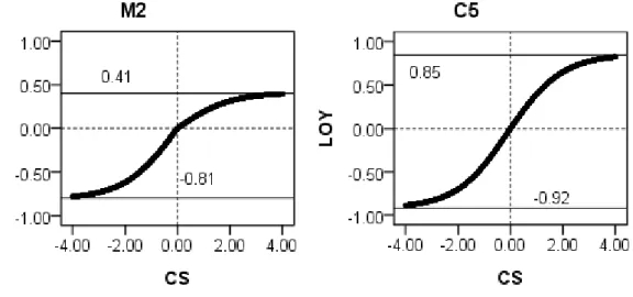
4.5. Estimated Functional Form
Figure 2 depicts the figure of estimated functional form of CS LOY. We observe
asymmetric responses in respective regimes and upper limits are smaller than negative of lower limits, implying loss aversion in relationship between satisfaction and loyalty. This is the most evident for M2 of mobile telecommunications as the difference is - 0.40 (= 0.41 - 0.81). The opposite situation happens for C5 in convenience stores, i.e., -0.07 (=0.92-0.85).
14
4.6. Distribution of Satisfaction Score
We express the levels of satisfaction and loyalty on 100-point scale as is usually reported in customer satisfaction index (CSI). The CSI score is calculated as the standardized factor scores for customer satisfaction by min[ ] 100
max[ ] min[ ] i i i i CS CS CS CS
. Figure 3 depicts the empirical distribution of respondent’s scores for each company. In the figure, the statistics of mean, median, and standard deviations as well as number of respondents are shown as legends. The score distributions are heterogeneous among companies. However, the distributions are relatively stable and symmetric since the difference of mean and median is small for every company. This is consistent with the study by Terui et al. (2011) on the ground of estimation after transformation of original categorical data to normal distributed data by data augmentation for Bayes modeling. Thus the sample mean would be reasonable estimate of CSI score even for nonlinear model.
Figure 3: Distribution of Satisfaction Score
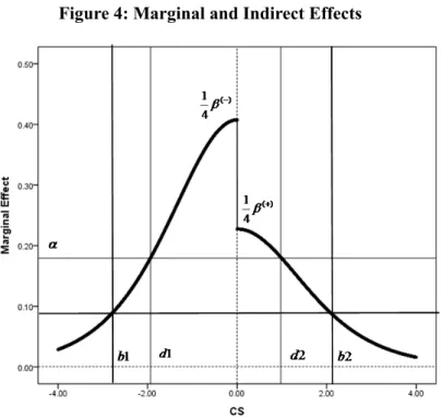
4.7. Marginal Effects and Indirect Effect of Satisfaction
Loyalty is determined not only by satisfaction, but also by the intention to recommend to others. According to the model (2), the marginal effects of satisfaction and recommendation intention are respectively measured by
ˆ
)
exp(
1
)
exp(
1
ˆ
)
exp(
1
)
exp(
ˆ
2 ) ( 2 ) (
i i i i i i i iRE
LOY
CS
CS
I
CS
CS
I
CS
LOY
(8)The marginal effect of satisfaction is not constant, changing with the level of satisfaction. In contrast, the marginal effect of recommendation intention is constant
ˆ
. Figure 4 depicts these effects. The marginal effect of satisfaction among dissatisfied customers (negative regime) is increasing up to1 ˆ
( )4
from the left, and then it is decreasing from
1 ˆ
( )4
toward zero.
15
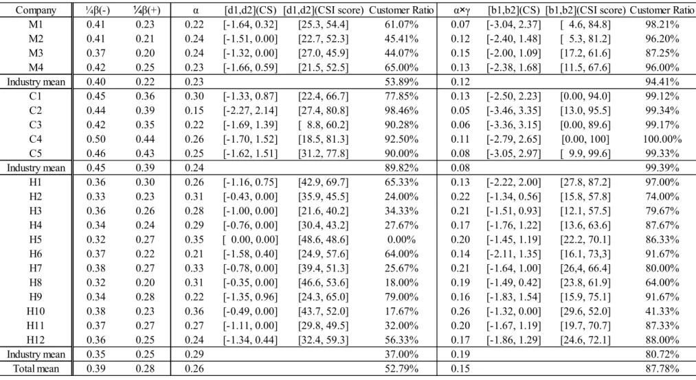
effects are positive over the domain of satisfaction for every company because of positive parameter estimates reported in Table 4. However, which is more influential depends on the level of satisfaction. According to the relation depicted in Figure 4, the satisfaction is more influential on loyalty than recommendation for the customers with the central level of satiation. The recommendation intention, in turn, is more effective for extreme customers. The interval of satisfaction where satisfaction is more important is reported as [d1, d2], and the transformed score by 100 points scale as [b1, b2] in Table 4. The percentage of customers who belong to this interval is also given as “Customer Ratio” and it shows that the satisfaction is more effective for 89% customers for convenient stores; 54% customers for telecommunication industry and 37% customers for hotel industry which has strong heterogeneity inside.
Figure 4: Marginal and Indirect Effects
Table 4: Marginal and Indirect Effects
Following the customer satisfaction model, RE is determined by CS as a structural equation
i i i
RE
CS
e
. (9)The indirect effect of CS to LOY is defined as marginal effect of estimated RE by CS,
RE
i
ˆ
CS
i,and it is given by
ˆ ˆ
. It means the effect of CS by way of RE to LOY.In (9), CS is assumed to have a positive effect on RE, and in fact
ˆ is estimated positive for every company. Then the indirect effect of CS by way of RE to LOY is interpreted as marginal effect of RE discounted by
ˆ. We also define the direct effect of CS as the marginal effect in (8), and we compare these effects over the domain of satisfaction. It is evident that direct effect is much more influential for loyalty by the interpretation of estimated indirect effects above. We define, similarly before, the interval where direct effect of CS is greater than indirect effect, and their “Customer Ratio”. These are reported in Table 4. It shows that the direct effect is most pervasive with over 99% customers in wider range of interval in convenience stores; in particular, it is dominant (100%) for the company C4. The hotels have rather significant impacts of indirect effect, 88% in average.16
The indirect effect is more important for the hotel H10 (41.33% customer ratio) and comparable for H8 (64%). The CS campaign leading to recommendation would be necessary for these
companies.
4.8. Managerial Implications
We consider two kinds of measure for managerial implications derived from our models. The first measure is the expected incremental loyalty that is defined by the expected values of incremental loyalty on unit change of satisfaction with respective to customer distribution on CSI scores. This measure is useful for overall evaluation of loyalty program when we assume that the firm approaches every customer. Under the limited budget for loyalty program, the second measure finds a customer segment optimizing the incremental loyalty.
(i) Expected Incremental Loyalty
According to satisfaction and loyalty scores obtained from the empirical study of our model, company managers can review their situations and formulate their strategies. First, the expected incremental loyalty (EIL) can be used to forecast future profitability of loyalty program by combining estimated response function and customers distribution over the same domain. Based on the empirical distribution of CSI scores in 4.6, we first set the cut-off point vector (0, 5, 10, 15, 20,..., 100) for CSI score dimension, and calculate the frequency of each cell to get the empirical distribution of CSI scores p
csi |data
, i=1,2,..., 20. Then we definea middle point vector (cs1 ,cs2 ,cs3 ...cs19 ,cs20) by (2.5, 7.5, 12.5,..., 97.5) for calculating estimate of marginal incremental loyalty, f '(csi) defined in (6). Then the EIL is formally defined by
)
|
(
)
(
'
20 1data
cs
p
cs
f
EIL
i i i
. (10)EIL shows the future profitability when loyalty program has a full access to their customers. Table 5 at the first column shows the measure of EIL for individual companies. The industry of convenience store has the highest EIL, and it will get the largest loyalty increment when the customers’ satisfaction level is improved. Another point is the difference between EIL and the band width given in Table 3.1. The band width of company M1 is a little lower than H11, having 1.27 and 1.28 respectively. However, M1 has higher EIL (0.2741) than H11 (0.2693). It means the extensible space of loyalty in M1 is not as wide as those in H11, however customers in M1 have more concentration around neutral point where it has the most
17
sensitive change of loyalty.
(ii) Targeted Customer Interval for Efficient Loyalty Program
Next, we consider a situation that company might just offer loyalty program to a limited proportion of customers due to their budget constraint. Our model provides the framework to consider how they should target some customers effectively subject to their budget for loyalty program. Assume that a company manager prospects that she/he is allowed to provide loyalty program for only 30% customers. Then the problem is to specify the set of customers under constrained optimization,
0
.
3
.
.
)
(
'
max
b i a CS CS iCS
CS
CS
P
t
s
CS
f
b a (11)Figure 5: Frequency and Increment Loyalty
We call the interval [CSa,CSb] 30% targeted customer interval (TCI), implying that the customer segment maximizes incremental loyalty induced by loyalty program. Figure 5 shows the smoothed frequency distribution of customer’s CSI scores on the left, and the marginal loyalty curve over CSI score dimension on the right. The customers whose CSI scores are located in this interval of [CSa,CSb] are most attractive to be targeted for increasing their loyalty. TCI is constructed in the same way as the highest probability density (HPD) region for Bayesian confidence interval. That is, we incorporate customers into TCI in order with higher incremental loyalty until the interval contains 30% customers.
Table 5: EIL and TCI
The second column of Table 5 shows the TCI for individual companies. Under the assumptions of limited access and identification of CSI scores of their customers, every company can find the customers to be targeted by their loyalty program.
18
5. Concluding Remarks
This study investigated the effects of customer satisfaction on loyalty by focusing on nonlinear characteristics represented as attainable limit of loyalty induced by satisfaction, asymmetric response between satisfied and dissatisfied customers, and not-constant marginal returns over the domain of satisfactions. There are a few extant works on investigating the relation between satisfaction and loyalty, in particular, and this is the first model to measure nonlinear relation based on a uniform measure of customer satisfaction index in terms of system equation by using structure that the loyalty is determined by customer satisfaction in the
connections of related other constructs. As is discussed in Fornell (1992), the investigation by using the system approach leads to higher reliability than the results obtained under the
perspective being limited to two variables.
We introduced hierarchical Bayes modeling for estimation to improve the measurement by considering company heterogeneity, to which identical model structure must be applied. In all, our study’s contributions to the modeling literatures are that (i) nonlinear term is embedded in the structural model of customer satisfaction index, and (ii) hierarchical Bayes modeling of nonlinear structural equation model for measuring customer satisfaction index to accommodate heterogeneity of surveyed companies. To our knowledge, this is the first study on nonlinear structural equation model which includes nonlinear term of endogenous latent variable. We propose an efficient algorithm of MCMC, i.e., multi-move sampler for latent variables by using Gibbs sampling.
In the empirical application, we compared comprehensive sets of specifications and the asymmetric nonlinear function with attainable limits is best supported by two kinds of criteria, goodness of fit measures and the number of significant parameter estimates. We obtained managerial implications for loyalty management such as attainable limits; customer’s loss aversion response; asymmetric marginal returns between satisfied and dissatisfied customers, i.e., increasing for dissatisfied customers and decreasing for satisfied customers, direct effect of customer satisfaction is more significant than recommendation in general. As managerial implications, we derived the measures for efficient loyalty program by combining information of estimated response curve of satisfaction to loyalty and empirical distribution of customers on the dimension of CSI scores under assumptions of fully and limited access to customers.
Other studies by using not loyalty but other outcome, for example, willingness to pay (Homburg et al., 2005), suggested the inverse S-shaped function which means having negligible
19
change for customers with medium level satisfaction in consistent with the concept of zone of tolerance. The inverse S-shaped function represents unrealistic situation since unlimited effect can be expected for highly satisfied (delighted) customers. Then the nonlinear function with neutral zone as well as attainable limits can be devised by modifying S-shaped function so that it has three regimes by two additional parameters which split the domain of satisfaction to plug zone of tolerance at the mid regime, and loss and gain regimes with attainable limits at the extremes. There is another nonlinear relationship between other constructs, for example, Mittal, Ross and Baldasare (1998) showed nonlinear relations from attribute performance (perceived quality in CSI), to satisfaction, suggesting inverse S-shaped function for it. The nonlinear CSI model including additional nonlinear terms is also possible. We leave these extensions for future research.
20
References
Andrews, F.M. (1984), “Construct Validity and Error Component of Survey Measures,” Public Opinion Quarterly, 48, 409-442.
Anderson, E. W., C. Fornell, and S. Mazvancheryl (2004), “Customer Satisfaction and Shareholder Value,” Journal of Marketing, 68, 172–185.
Anderson, Eugene W. and Vikas Mittal (2000), “Strengthening the Satisfaction-Profit Chain,” Journal of Service Research, 3 (2), 107-120.
Anderson, Eugene W. and Linda C. Salisbury (2003), “The Formation of Market-Level Expectations and Its Covariates,” Journal of Consumer Research, 30 (June), 115-124. Bloemer, J. and K. de Ruyter (1998), “On the Relationship between Store Image, Store
Satisfaction and Store Loyalty,” European Journal of Marketing, 32, 499–513. Bolton, Ruth N. and Katherine N. Lemon (1999), “A Dynamic Model of Customers’
Usage of Services: Usage as an Antecedent and Consequence of Satisfaction,” Journal of Marketing Research, 36 (2), 17-186.
Bowman, D. and D. Narayandas (2004), “Linking customer management effort to customer profitability in business markets,” Journal of Marketing Research, 41, 433–447
Cooil, B., T.L. Keiningham, L. Aksoy and M. Hsu (2007), “A longitudinal analysis of customer satisfaction and share of wallet: investigating the moderating effect of customer
characteristics,” Journal of Marketing, 71, 67–83.
Dong, Songting, Min Ding, Rajdeep Grewal, and Ping Zhao (2011), "Functional Forms of the Satisfaction-Loyalty Relationship," International Journal of Research in Marketing, 28 38- 50.
Eisenbeiss, M., M. Cornelißen. K. Backhaus and W.D. Hoyer (2014), “Nonlinear and
asymmetric returns on customer satisfaction: do they vary across situations and consumers?,” Journal of the Academy of Marketing Science, 42, 242–263.
Fornell, C. and B. Wernerfelt (1988), “A model for customer complaint management,” Marketing Science, 7, 287-298.
Fornell, C. (1992), “A National Customer Satisfaction Barometer: The Swedish Experience,” Journal of Marketing, 56, 1–21.
21
Modeling,” Sociological Methods and Research 20, 291-320.
Fornell, C., M.D. Johnson, E.W. Anderson, J. Cha, and B.E. Bryant (1996), “The American Customer Satisfaction Index: Nature, Purpose, and Findings,” Journal of Marketing, 60, 7– 18.
Fornell, C., R.T. Rust, and M.G. Dekimpe (2010), “The Effect of Customer Satisfaction on Consumer Spending Growth,” Journal of Marketing Research, 47, 28–35.
Homburg, C., N. Koschate and W.D. Hoyer (2005), “Do satisfied customers really pay more? A study of the relationship between customer satisfaction and willingness to pay,” Journal of Marketing, 69, 84–96.
Howard, J.A. and J.N. Sheth (1969), The Theory of Buyer Behavior, New York: John Wiley & Sons. Inc.
Gupta, Sunil and Valarie Zeithaml (2006), “Customer Metrics and Their Impact on Financial Performance,” Marketing Science, 25 (6), 718-739.
Gupta, Sunil, Donald R. Lehmann, and Jennifer Ames Stuart (2004), “Valuing Customers,” Journal of Marketing Research, 41 (1), 7-18.
Jones, T. O. and W. Earl Sasser (1995), “Why Satisfied Customers Defect,” Harvard Business Review, 73, 88–99.
Khaneman, Daniel and Amos Tversky (1979) "Prospect Theory: An Analysis of Decision Under Risk," Econometrica, 47, 2, 263-291
Keiningham, T. L., Perkins-Munn, T. and Evans, H. (2003), “The impact of customer satisfaction on share-of-wallet in a business-to-business environment,” Journal of Service Research, 6, 37–50.
Kumar, V., Ilaria Dalla Pozza and Jaishankar Ganesh (2013), “Revisiting the Satisfaction– Loyalty Relationship: Empirical Generalizations and Directions for Future Research”, Journal of Retailing, 89 246-262.
Lee, S. Y. (2007), Structural Equation Modeling: A Bayesian Approach, Wiley, New York. Mittal, V. and W. A. Kamakura (2001), “Satisfaction, Repurchase Intent, and Repurchase
Behavior: Investigating the Moderating Effect of Customer Characteristics,” Journal of Marketing Research, 38, 131–142.
Mittal, V., W.T. Ross, and P.M. Baldasare (1998), “The Asymmetric Impact of Negative and Positive Attribute-Level Performance on Overall Satisfaction and Repurchase Intentions,”
22
Journal of Marketing, 62 (January), 33–47.
National Quality Research Center (NQRC; 2005), “American Customer Satisfaction Index (ACSI): Methodology Report,” Stephen M. Ross School of Business at the University of Michigan.
Ngobo, Paul-Valentin (1999), “Decreasing Returns in Customer Loyalty: Does It Really Matter to Delight the Customers?”, Advances in Consumer Research, 26 (1), 469–76.
Oliver, R.L. (1980), “A Cognitive Model of the Antecedent and Consequences of Satisfaction Decisions,” Journal of Marketing, 17, 460–469.
Oliver, R.L. (1981), “Measurement and Evaluation of Satisfaction Process in Retail Setting,” Journal of Retailing, 17, 460–469.
Terui, N., S. Hasegawa, T. Chun, and K. Ogawa (2011), “Hierarchical Bayes Modeling of the Customer Satisfaction Index,” Service Science, 3(2), 127–140.
Westbrook, R.A. and M.D. Reilly (1983), “Value-Percept Disparity: An Alternative to the Disconfirmation of Expectation Theory of Consumer Satisfaction,” Advances in Consumer Research, 10, 256-261.
23
Figure 1: Linear and Nonlinear CSI Model
(a) Asymmetric Linear (b) Asymmetric Logit
24
Figure 2: Estimated Functional Form and Upper and Lower Limits
25
Figure 4: Marginal and Indirect Effects
26
Table 1:Model Comparison: DIC and log of Marginal Likelihood
Table 2: The Effect of HB modeling on Estimate of Path Coefficients
The number means the percentage of significant estimates in the model. The ratio is given in parenthesis.
Symmetric Asymmetric
Threshold Symmetric Asymmetric Threshold
DIC
238539.1
234960.5
234912.3
234963.2
234908.7
234908.5
234937.7
LML
-98516.1
-96844.0
-96577.7
-96578.3
-96568.3
-96575.5
-96570.8
HB
Linear
Logit
Independent
IndependentSymmetric Asymmetric Threshold Symmetric Asymmetric Threshold Total 14.29% (27/189) 8.47%(16/189) 8.10%(17/210) 7.79%(20/231) 6.88%(13/189) 6.19%(13/210) 6.06%(14/231) Mobile Telecommunication 19.44%(7/36) 5.56%(2/36) 5%(2/40) 11.36%(5/44) 5.56%(2/36) 5%(2/40) 4.55%(2/44) Convenience stores 4.44%(2/45) 2.22%(1/45) 2%(1/50) 1.82%(1/55) 2.22%(1/45) 2%(1/50) 1.82%(1/55) Hotels 16.67%(18/108) 12.04%(13/108) 11.67%(14/120)10.61%(14/132) 9.26%(10/108) 8.33%(10/120) 8.33%(11/132) HB Linear Logit
27
Table 3.1: Parameter Estimates (Company Level)
Table 3.2: Parameter Estimates (Industry Level)
The posterior mean of parameter estimate, and 95% HPD region are given for respective parameters. The table contains the column for band width
1
( )1
( )2
2
for attainablelimits.
Company β(-) HPD β(+) HPD Pr{β(-) >β(+)} Band Width α HPD
M1 1.63 [0.98, 2.28] 0.91 [0.29, 1.56] 91.12% 1.27 0.22 [0.12, 0.33] M2 1.62 [1.06, 2.18] 0.82 [0.25, 1.41] 95.54% 1.22 0.24 [0.15, 0.34] M3 1.46 [0.82, 2.04] 0.82 [0.19, 1.44] 89.28% 1.14 0.24 [0.15, 0.34] M4 1.68 [1.09, 2.28] 0.99 [0.42, 1.56] 92.34% 1.33 0.23 [0.13, 0.33] Industry mean 1.60 0.88 92.07% 1.24 0.23 C1 1.79 [1.18, 2.37] 1.43 [0.85, 2.01] 77.56% 1.61 0.30 [0.21, 0.39] C2 1.75 [1.25, 2.26] 1.57 [1.06, 2.12] 66.70% 1.66 0.15 [0.07, 0.23] C3 1.70 [0.99, 2.34] 1.40 [0.72, 2.08] 70.92% 1.55 0.22 [0.11, 0.35] C4 2.00 [1.46, 2.54] 1.77 [1.23, 2.37] 69.46% 1.89 0.26 [0.17, 0.35] C5 1.84 [1.30, 2.37] 1.71 [1.19, 2.25] 61.88% 1.78 0.25 [0.16, 0.35] Industry mean 1.81 1.58 69.30% 1.69 0.24 H1 1.42 [0.97, 1.88] 1.19 [0.74, 1.66] 75.38% 1.31 0.26 [0.16, 0.37] H2 1.31 [0.83, 1.80] 0.93 [0.42, 1.44] 85.44% 1.12 0.31 [0.21, 0.44] H3 1.44 [1.06, 1.83] 1.06 [0.63, 1.50] 89.36% 1.25 0.28 [0.20, 0.44] H4 1.34 [0.92, 1.75] 0.95 [0.54, 1.38] 89.58% 1.15 0.29 [0.20, 0.39] H5 1.28 [0.77, 1.76] 1.10 [0.57, 1.63] 68.60% 1.19 0.35 [0.23, 0.46] H6 1.48 [1.08, 1.91] 0.87 [0.45, 1.28] 97.66% 1.18 0.21 [0.12, 0.31] H7 1.54 [1.09, 2.02] 1.06 [0.58, 1.54] 91.78% 1.30 0.33 [0.23, 0.45] H8 1.26 [0.75, 1.76] 0.79 [0.26, 1.30] 89.30% 1.03 0.31 [0.20, 0.42] H9 1.36 [0.91, 1.83] 1.11 [0.63, 1.63] 77.10% 1.24 0.22 [0.13, 0.34] H10 1.54 [1.06, 2.05] 0.92 [0.41, 1.42] 95.36% 1.23 0.36 [0.25, 0.48] H11 1.47 [1.04, 1.92] 1.10 [0.62, 1.57] 87.08% 1.28 0.27 [0.17, 0.38] H12 1.44 [1.03, 1.89] 0.99 [0.54, 1.46] 91.80% 1.22 0.24 [0.15, 0.34] Industry mean 1.41 1.01 86.54% 1.21 0.29 Total mean 1.54 1.12 83.49% 1.33 0.26
28
Table 4: Marginal and Indirect Effects
Company ¼β(-) ¼β(+) α [d1,d2](CS) [d1,d2](CSI score) Customer Ratio α×γ [b1,b2](CS) [b1,b2](CSI score) Customer Ratio
M1 0.41 0.23 0.22 [-1.64, 0.32] [25.3, 54.4] 61.07% 0.07 [-3.04, 2.37] [ 4.6, 84.8] 98.21% M2 0.41 0.21 0.24 [-1.51, 0.00] [22.7, 52.3] 45.41% 0.12 [-2.40, 1.48] [ 5.3, 81.2] 96.20% M3 0.37 0.20 0.24 [-1.32, 0.00] [27.0, 45.9] 44.07% 0.15 [-2.00, 1.09] [17.2, 61.6] 87.25% M4 0.42 0.25 0.23 [-1.66, 0.59] [21.5, 52.5] 65.00% 0.13 [-2.38, 1.68] [11.5, 67.6] 96.00% Industry mean 0.40 0.22 0.23 53.89% 0.12 94.41% C1 0.45 0.36 0.30 [-1.33, 0.87] [22.4, 66.7] 77.85% 0.13 [-2.50, 2.23] [0.00, 94.0] 99.12% C2 0.44 0.39 0.15 [-2.27, 2.14] [27.4, 80.8] 98.46% 0.05 [-3.46, 3.35] [13.0, 95.5] 99.34% C3 0.42 0.35 0.22 [-1.69, 1.39] [ 8.8, 60.2] 90.28% 0.06 [-3.36, 3.15] [0.00, 89.6] 99.17% C4 0.50 0.44 0.26 [-1.70, 1.52] [18.5, 81.3] 92.50% 0.11 [-2.79, 2.65] [0.00, 100] 100.00% C5 0.46 0.43 0.25 [-1.62, 1.51] [31.2, 77.8] 90.00% 0.08 [-3.05, 2.97] [ 9.9, 99.6] 99.33% Industry mean 0.45 0.39 0.24 89.82% 0.08 99.39% H1 0.36 0.30 0.26 [-1.16, 0.75] [42.9, 69.7] 65.33% 0.13 [-2.22, 2.00] [27.8, 87.2] 97.00% H2 0.33 0.23 0.31 [-0.43, 0.00] [35.9, 45.5] 24.00% 0.22 [-1.34, 0.56] [15.8, 57.8] 74.00% H3 0.36 0.26 0.28 [-1.00, 0.00] [21.6, 40.2] 34.33% 0.21 [-1.51, 0.93] [12.1, 57.5] 79.67% H4 0.34 0.24 0.29 [-0.76, 0.00] [30.4, 43.2] 27.67% 0.17 [-1.76, 1.22] [13.6, 63.6] 87.67% H5 0.32 0.27 0.35 [ 0.00, 0.00] [48.6, 48.6] 0.00% 0.20 [-1.45, 1.19] [22.2, 70.1] 86.33% H6 0.37 0.22 0.21 [-1.58, 0.40] [24.9, 57.6] 64.00% 0.14 [-2.11, 1.35] [16.1, 73,3] 91.67% H7 0.38 0.27 0.33 [-0.78, 0.00] [39.4, 51.3] 25.67% 0.21 [-1.64, 1.00] [26,4, 66.4] 80.00% H8 0.32 0.20 0.31 [-0.35, 0.00] [46.6, 53.6] 18.00% 0.19 [-1.49, 0.42] [23.8, 61.9] 64.00% H9 0.34 0.28 0.22 [-1.35, 0.96] [24.3, 65.0] 79.00% 0.16 [-1.83, 1.54] [15.9, 75.1] 91.67% H10 0.38 0.23 0.36 [-0.49, 0.00] [43.7, 52.0] 17.67% 0.26 [-1.32, 0.00] [29.6, 52.0] 41.33% H11 0.37 0.27 0.27 [-1.11, 0.00] [29.8, 49.5] 32.00% 0.20 [-1.67, 1.19] [19.7, 70.7] 87.33% H12 0.36 0.25 0.24 [-1.34, 0.44] [32.4, 59.3] 56.33% 0.17 [-1.86, 1.29] [24.6, 72.1] 88.00% Industry mean 0.35 0.25 0.29 37.00% 0.19 80.72% Total mean 0.39 0.28 0.26 52.79% 0.15 87.78%
29
30
Appendix A: Full Description of Model and Inference Procedure
The CSI model assumes six latent variables and these are extracted by 17 questions of survey. For the vector of question items
y
i
(
y
1 , , 17i…y
i)
', which are ordered categorical variables, we first transform them into continuous datax
i
(
x
1 , , 17i…x
i)
' following normal distribution. This transformation is conducted by data-augmentation when… ' 1 , , 17
(
)
i i i
y
y
y
is given at the conditional posterior density in Appendix B.The structural equation model has measurement model to extract the latent variables from data, and structural model which describes the relation between latent variables. Then we set the measurement model for by factor model and we define the structure on the factors as structural model.
(i) Measurement model
The observable vector of
x
i
(
x
1 , , 17i…x
i)
' has a factor analytic representation with six factors,
1, ...
i i i
x
i
n
(A1)where represents the factor loading matrix,
i
( , ,
i 1i 2i,...,
5i)
' is factor score vector for represents. The error term vector
i
(
1 , , 17i… i)
' is assumed to follow
17
~
0,
i
N
where
diag
1...,
17
. (ii) Structural modelThe structural equation model assumes that the factor scores have the relation each other in terms of set of equations:
Perceived Quality: (A2) Perceived Value: (A3)
' 1 2 5
( ,
,...,
, )
i i i i i
ix
i ' 1 2 5( ,
,...,
, )
i i i i i
1 16 1
2 21 1 26 2
31
Customer Satisfaction: (A4) Recommendation Intention:
4
43 3
4 (A5)Customer Loyalty:
(A6)
where
1,...,5
' ~N5
0, ,
diag
1,...,
5
.More specifically, the model describes that customer expectation drives perceived quality
1 and perceived value
2. These three latent variables next generate customersatisfaction
3, which directly affects recommendation intention
4 and customer loyalty
5. Equation (A6) indicates the extension of this study.Bayesian Inference of Nonlinear SEM
The structural models (A2)-(A6) play a role of prior for the likelihood defined by the measurement model (A1) for Bayesian inference. The joint prior density of
'1, 2,..., 5,
is decomposed by using their recursive relation between endogenous latent variable by
1|
2| ,1
3| , ,1 2
4| 3
5| ,3 4
p
p
p
p
p
p
p
(A7)On the other hand, we denote the likelihood function for conditional on parameters and data x as , then full conditional posterior density is as follows: (i)
[ ]
| , | , p
x
p
p x
(ii) (iii) 3 31 1 32 2 36 3
( ) ( ) 5 53 53 54 4 5 3 31
1
1
1
1
1 exp
2
1 exp
2
I
I
1, ,...,2
5
,
1| ,
n i| ,
i ip x
p x
[ ]1
1| , , 1| | , p
x
p
p x
[ 2]
2| , , ,1 2| ,1 | , p
x
p
p x
32 (iv)
[ ]3
3| , , , ,1 2 3| , ,1 2 | , p
x
p
p x
(v) (vi)
[ 5]
5| ,3 4 , 5| ,3 4 | , p
x p
p x
where means the part of joint likelihood regarding the latent variable z.
These conditional posteriors are analytically evaluated to be normal distribution since both prior and likelihood functions are normal density.
Then, staring from initial value , we iterate the Gibbs sampling from the conditional posterior density to obtain the joint posterior density . This is a single move-sampler for MCMC.
The multi-move sampler is available for our model by the use of recursive system of CSI model to derive more efficient algorithm by using linearity of subsystem on
1 1, , , ,2 3 4 '
. That is, we set the joint prior density by
1( | , )
5 3 4p
p
p
(A8)and the conditional posterior density is obtained by multi-move sampler for
1 following by Lee (2007) since full conditional posterior density is as follows:(i)
[ 1]
1| , 1 | , p
x
p
p x
(ii)
[ 5]
5| ,3 4 , 5| ,3 4 | , p
x p
p x
The details of algorithm are described in Appendix B. Appendix B: MCMC Algorithms
The prior setting and conditional posterior density are described in this appendix for our model. The measurement model connecting observed data and latent variables in the form of factor model (A1), and structural model relating latent variables (A2)-(A6) are compactly written by
[ 4]
4| , ,3 4| 3 | , p
x
p
p x
[ ] | , z p x
(0) (0) (0) (0) (0) ' 1 2 5(
,
,...,
,
)
| ,
p
x
33
~ (0,
~ (
;
)
),
0,
~ (0,
)
;
hi h hi hi hi h hi h hi h hi h hi h hi hi h hi hix
N
N
N
(B1)
( ) ( ) 53 53 54 3 3 5 4 5 1 1 1 1 1 1 exp 2 1 exp 2 h h h h h h i h h I I
(B2) (1) Prior DensityThe diffuse priors are set on the model parameters, and these are shown in next table:
Parameter Setting 0 0 ~ ( , ) hj IG
R
01
3,
0
1
,
1
~
|
|
D
V
vec
N
V
vec
V
0
HZ,
D
I
HH
100
) , ( ~ 0 0 IG v V Vhv
0
2
,
V
0
2
where is the th row of ,
k is th element of (k 1, ,17), is theth row of , and is th element of . H means the number of
companies, and
V
h is covariance matrix of path coefficient in structure model of company h. L is the number of path coefficients. Z is the number of variables of attributes for company, and we use industrial dummy variables for this.0 0