空間2次元のリーゼガング現象とその数理(第2回生物数学の理論とその応用)

A Mathematical

Aspect

for Liesegang Phenomena

in

two space dimensions

(

空間

2

次元のリーゼガング現象とその数理

)

広島大学大学院理学研究科数理分子生命理学専攻

1 大西

勇 (Isamu Ohnishi)

Dept.

of

Mathematical and Life

sciences,

Graduate School

of

Science,

Hiroshima

University

1

Introduction

$\mathrm{H}^{\backslash }1$: Liesegangband [1]

$\mathrm{H}2$: Liesegang ring [2]

We

can see

very beautiful pattern formation

as snow

in a single crystal. In

case of

mak-ing precipitation after crystallization, there

are some cases

where verystrikinglyregular

macro-scopicpatterns

can

be

seen.

Especially,it iswell-known that spacio-temporallyperiodic patterns

emergein reaction-diffusion processwith precipitation in gel, if there is adequate difference of initial densities betweentwo chemical reaction substances. In Germany, Linge first discovered

this phenomena in 1855, and in 1896 Professor R.E.Liesegang studied it first

as

a science. In

vitro,

we can

find band pattern andring pattern inone space dimension andtwo space

dimen-sions, respectively (Fig. 1 and Fig. 2). These

are called

Liesegang band and Liesegang ring,

respectively,after ProfessorLiesegang. Theinterestingpointis that such

a

spacio-temporal

dis-continuous pattern is formed in spiteofchemical reaction

occurs

continuously, and this patter

$\underline{\mathrm{s}\mathrm{a}\mathrm{t}\mathrm{i}\mathrm{s}\mathrm{f}\mathrm{i}\mathrm{e}\mathrm{s}}$

very

strikingly regular laws(timelaw, spacing law, and

width

law).

iThisnoteisbasedonthejoint work with ProfessorM. Mimura inMeiji Universityand Dr. D. Ueyama in

Hiroshima University, although, if therearemistypesormistakes undermisunderstanding,then all of themare

duetotheauthor. If youhaveaquestion,would youplease mail himtothe address: [email protected]&

In this note, we report

our

recent studies about such very interesting problem of Liesegang phenomena.

2

History

There have been made of tons of researches about Liesegang phenomena since the previous

century. Forexample, there

are

$\mathrm{A})\mathrm{T}\mathrm{h}\mathrm{m}\mathrm{r}\mathrm{y}$of pre-nucleation: 1. super-saturationtheory ([6], [7])

2. diffusiontheory ([8])

3. diffusion

wave

theory ([9])

4.adsorption theory ([10])

5. membranetheory ([11])

$\mathrm{B})\mathrm{T}\mathrm{h}\infty \mathrm{r}\mathrm{y}$ of post-nucleation:

1.theoryof

colloid

growth and dissoluton ([3],[12])

2. theoryof

colloid

coherence ([13]).

In the former

group

oftheories, they consider that positionofpattern is determinedjust when

the chemical reaction

occures

before nucleation. This is very old way of thinking about this

phenomena. On theother hand, in thelatter group oftheories, they consider ofthepositionof

pattern is decided after nucleation. There

are

some

facts which cannot be explained from the

former theories; for example, spiral structure

or

double periodicstructure. Briefly speaking,

we

cannot understandthatthe followingproperties:

1) Colloid particles

can

be

seen

inwiderareabefore precipitation,

2) Band

or

ring pattern

can

be formed if

colloid

solution with

a

mean radius of particles

touches

another

with

another

mean

radius,

3) Gavityaffects the position ofpattern,

4) Subring pattern

can

beoftenseen,

5) The Second structure canbe made in

a

ring

or

bandpattern,

6) Spacialbifurcation oftenoccurs,

7) Spacinglaws

can

bestochastic ifthedensity difference is less.

Keller-Rubinow model is famousin the super-saturation theory. Inthenextsection webriefly

statesomenumericalsimulations and insufficientpoints inthis$\mathrm{m}o\mathrm{d}\mathrm{e}\mathrm{l}$

.

3

Super-saturation

theory

3.1

Summary

1) Precipitation

occurs

ifthedensityreach the super-saturationdensitybigger than the satu-ration density,

2) Reaction speed is much faster than diffusion speed,

and tried to explain Liesegangphenomena. Especially, accourding to themodel, the

discontinu-ous

presipitation

emerges.

In the nextsection,

we introduce

Keller-Rubinow model in detail to

makenumericalsimulations.

$\wedge\S V3$ $\frac{\mathrm{C}}{\infty}$ $\cup$ $. \frac{.\mathcal{Q}\mathrm{C}}{\mathrm{g}}$ $\overline{\mathrm{C}}$ $\not\in \mathrm{S}$

$\mathrm{H}3$: Super-saturationtheory [3]

3.2

Keller-Rubinow model

In 1981,Professors J.B.Keller and S.I.Rubinow made the model called Keller-Rubinow model

nowaday,with effect ofadsorption

of

colloid combined withthesuper-saturationtheory. This is

thefollowing:

$v_{A}A^{+}+v_{B}B^{-}\Leftrightarrow v_{C}Ck$

, (1)

with$k_{+},$ $k$-chemicalreactionconstants,$v_{A},$ $v_{B},$ $v_{B}$,stoichiometriccoefficients,$qP$precipitation

rate, $q$ precipitation coefficient. Here,

we

make $v_{A}=v_{B}=v_{C}=1,$ $k_{-}=0$

.

We

can

make this

be the following system of partialdifferentialequations:

$\{$ $at=D_{A}\Delta a-kab$, $b_{t}=D_{B}\Delta b-kab$, $c_{t}=D_{C}\Delta c+kab-qP(c, d)$

,

$d_{t}=qP(c,d)$, (3)

where, $a,$ $b,$ $c,$ $d$

are

density of each ingredient, $D_{A},$ $D_{B},$ $D_{C}$

are

diffusion

coefficients, _{$k=k_{+}$}

chemical reactionconstant. The diffusion of$D$

can

benegligible. _$P(c,d)$ has thefollowingform:

$P(c,d)=\{$ $(c-C_{a})_{+}$

,

if

$c>C_{\epsilon}$

or

$d>0$ $0$, otherwise

(4)

where$C_{a},$ $C_{s}$

are

saturation density and super-saturation density of$C$, respectively $(C_{s}>C_{a}>$

$0)$

.

(Fig. 4)

$\mathrm{H}4$: Precipitation $P(c, d)$

3.3

Numerical simulation

3.3.1 One

space

dimension

The initialconditon is

$a(\mathrm{O}, x)=c(\mathrm{O},x)=d(\mathrm{O}, x)=0,$ $b(\mathrm{O},x)=B_{0}$, (5)

andthe boundarycondition is

$a(t,\mathrm{O})=A_{0},b_{x}(t,0)=c_{x}(t,0)=0,0<t<T$

(6)

$a_{x}(t, L)=b_{x}(t,L)=c_{x}(t, L)=0,0<t<T$

with $A_{0}>>B_{0}>0$

.

(parameters

are

the followings: $A_{0}=10.0,$ $B_{0}=1.0,$ $D_{A}=D_{B}=D_{C}=$

0.001, $C_{a}=0.2,$ $C_{\delta}=0.8,$ $k=50.0,$$q=50.0,L=1.5$ )

The result is Fig. 7. Spacing law and time law

are

satisfied enough very well, but width

precipitation

occurs

discretely, although it is not enough inpointof view

of

width of

precipita-tion. But

Keller-Rubinow

model issimple andgood forunderstanding the mechanismby which precipitation

occurs

discretely and satisfies timelaw and spacing law. In fact, we havealready

given

a

mathematically rigorous proofwhich

ensure

Keller-Rubinow modelhas

a

mathematically

rigorous solution satisfying time law and spacing law under natural assumptions. See indetail

[15], [16], [17], and [18].

$X_{\prime\iota_{1\prime}},\cdot.*\cdot’..\cdot\ldots:**\cdot...\cdot...\ldots..\cdot|u^{--}\prime_{\overline{\mathrm{m}u\cdot\cdot u}\cdot \mathrm{b}\cdot l\cdot\cdot\cdot\cdot u}’\overline{\wedge\neg^{r}\prime}$

$X_{N}$

$\mathrm{H}5$: spacinglaw

$’.’ !.\cdot\cdots\cdots\cdots\cdots\cdots\cdot\cdots\cdots\cdot\cdot\cdots\cdots\cdot\cdot\cdots\cdots\cdots\cdot\cdots\cdot\cdot r-\overline{--\rfloor^{1}\}}$

.

$|_{1}^{\mathrm{t}}$ $\sqrt{t},$$\cdot:$.

.

$.\prime\prime|.\cdot\bullet \mathrm{i}_{;P_{-\dot{u}\overline{\mathrm{r}}}}\ldots.\ldots\ldots$ .-.. $-*\cdot u\rfloor$ $11$ $X_{N}$

$\mathrm{H}6$: timelaw

4

Theory

of

colloid growth

and dissolution

4.1

Kai’s theory

Professor

S.

Kai (Kyushu University) made

a

theorywhichexplainedmechanismof Liesegang

phenomena in view of colloid growth and dissolution in [4]. We

use

it to try to make

a new

mathematical

model ofLiesegang phenomena.

pa

8:

colloid growthand

dissolution

4.2

Simple application of Kai

$‘ \mathrm{s}$

theory

We consider about the followingsystem ofequations:

$v_{A}A^{+}+v_{B}B^{-}\Leftrightarrow v_{C}Ck$ ₍₇₎ $Carrow DP$ (8) $\{$ $a_{t}=D_{A}\Delta a-kab$, $b_{t}=D_{B}\Delta b-kab$, $c_{t}=D_{C}\Delta c+kab-P$

,

$d_{t}=P$, (9)

where

we

rewrite the term$P$

as

follows:

$P=q \frac{\partial}{\partial t}(\frac{4}{3}\pi R^{3})$

(10)

$R$ : radius ofcolloidparticle, _$q,$$M$: constants, $C_{a}(R)$ is the Gibbs-Thomson formula, which isexacly the following;

$C_{a}(R)=C_{e}(1+ \frac{\alpha}{R})$

$\alpha=\frac{2\sigma V}{k_{B}T}$

Here

$C_{\mathrm{e}}$ :

saturation

density

of

the idealparticle

with radius

$\infty$, $\sigma$

:

surface

energy,

$V$: volume, $k_{B}$ : Boltzmann constant, $T$: templature.

4.3

Numerical

simulation

4.3.1 One space dimension

We make comuter simulation withparameters: $A_{0}=10.0,$ $B_{0}=1.0,$ $D_{A}=D_{B}=D_{C}=0.001$, $k=20,$ $q=0.5,$ $M=1.\mathrm{O},$ $\alpha=0.05,$ $L=10.\mathrm{O}$

.

$\mathrm{H}9$:

One space

dimension

We try to verify the three charasteristic lawsofLiesegang phenomena. Timelaw and spacing

law

are

satisfied verywell likethe

case

of

Keller-Rubinow

model. But widthlaw is notsatisfied,

$\mathrm{n}"\ldots\ldots..-..---\cdots\wedge\cdots\cdot-\sim\cdots\cdots\cdot\cdots\cdot\cdots\ldots\ldots.’\ldots\ldots..\cdots\ldots\ldots\ldots...\ddot{\acute{\ddot{\ddot{\ddot{\ddot{\dot{\mathrm{r}}}}}}}},.:..\cdot.\cdots.\urcorner|$

$X_{N+1^{(:_{k\prime\cdot\cdot\cdots\cdots\cdot\cdot:^{-\cdots\ldots\ldots\sim\ldots\iota\ldots\ldots\ldots\ldots\ldots\ldots..l.\ldots\ldots\ldots\ldots\ldots.\prime}j|\dot{u}}|}}\ldots,..\cdot\ldots..\ldots|\ldots..\bullet\nearrow\cdot\bullet’|\ddot{n}\ldots\ldots\ldots\ldots\ldots\ldots\ldots\ldots\ldots\ldots..A\ldots\ldots..\rfloor$

$X_{N}$

$\mathrm{H}10$: spacinglaw $\mathrm{H}11$: timelaw

4.3.2 Two

space

dimensions

We make two

sapce dimensional

simulation to get Fig. 12.

$t=50.0$ $t=1240.0$

$\mathrm{H}12$: Two space dimensions

In thismodel,

we can

make

simulations of

thetwodimensinalringpattern, althoughthe patterns

dissapearafter much time goesby. Theresultisbetterthanin the

case

of Keller-Rubinowmodel,

but

we

cannot be satisfied with it. In the next section

we

improvethis model to get the result

much better to discuss about theinterestingview pointsofLiesegang phenomena.

5

Improvement

of the model

We improvethe modelto set the ringpattern fixed adequately. Let

us

$\mathrm{c}o$nsiderthefollowing

6

Improved

model

$\{$ $a_{t}=D_{A}\Delta a-kab$ $b_{t}=D_{B}\Delta b-kab$ $c_{t}=D_{C} \Delta c+kab-q\frac{d}{dt}(\frac{4}{3}\pi R^{3})$ $R_{t}=F(c, R)$ (11) $F(c, R)=\{$ $\frac{\Lambda f}{R}(c-\frac{\alpha}{R})_{+}$ if$R_{1}<R$ $\frac{M}{R}(c-\frac{\alpha}{R})$ if$R_{0}<R\leq R_{1}$ $\frac{M}{R_{0}}(c-\frac{\alpha}{R_{0}})$ if$0\leq R\leq R_{0}$ $-hR$ if$R<0$

(12)

Here

$R_{0}$ : minimum radius of colloidparticle, $R_{1}$

:

minimum radius of precipitated colloidparticle

$q,$$h$: positive constants, $h\gg 1$ and $f(x)_{+}$ satisfies $f(x)_{+}=\{$ $f(x)$ $0$ if$f(x)\geq 0$ if$f(x)<0$

7

Numerical simulation

7.1

One space dimension

$\mathrm{Q};-\mathrm{T}\mathrm{l}\mathrm{l}\mathrm{a}*:-\mathrm{n}\mathrm{r}\mathrm{a}\mathrm{o}$

”$1+;_{\mathrm{Q}}\mathrm{f}-11_{\cap \mathrm{m}}\mathrm{i}\mathfrak{n}\sigma(\mathrm{F}\mathrm{i}\sigma 1?)$

.

Pa

13: simulation ofthe model (11), (12)

The threelaws arethe followings (Fig. 14, Fig. 15,andFig. 16):

$X_{N}$

$\mathrm{H}14$: spacing law _{$\mathrm{H}15$}: time law

$1\mathcal{V}_{N}^{\cdot}.\alpha_{r_{}}..,,-\sim.-...-....--\alpha_{1}rightarrow;\wedge u:^{j}::|.||\overline{\wedge|}1$

$.\mathrm{u}_{\mathfrak{l}}\backslash ,,.‘.(-_{:--arrow-*----\cdot\cdot\infty\cdot\cdot r}1|\sim---[]^{\sim m}-\mathrm{a}x^{1}$

.

$X_{N}$

7.2

Two

space

dimensions

The result is Fig. 17. ($A_{0}=10.0,$ $B_{0}=1.0,$ $D_{A}=D_{B}=D_{C}=$ 0.001, $k=20,$ $q=0.5$,

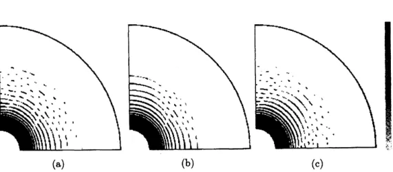
$M=1.0,$ $\alpha=0.04,$$R_{0}=0.1,$ $R_{1}=1.0,$$R=2.0)$ (a) $\ovalbox{\tt\small REJECT}_{\Psi^{:}}u\mathfrak{B}$

1.0

o.o

(b)

$\mathrm{H}17:(\mathrm{a})$

Chemical

experiment, (b) Numerical simulation

By use of the improved model, we realize the similar pattern to the real chemical experiment

unlike in the caseof Keller-Rubinow model. We make anobservation of the pattern in details

(Fig. 18).

$\mathrm{t}=185.8$ $\mathrm{t}=187.825$ $\mathrm{t}=194.425$ $\mathrm{t}=196.125$

@18:

Process ofmaking ring 17(b)

We can consider of this model

as

much better than the previous

ones.

Therefore, we try to

make

more

simulation to realize otherpatternsin two space dimensions introducedinSection 2.

$|_{4}* \int_{\mathrm{B}}\#$

1.0

o.o

(a) (b)

$\mathrm{H}19:(\mathrm{a})$ Realexperiment, (b) Numericalsimulation

Thering patternis madecut accourding to going awayfrom the center,which is similarto the

real chemical expariment. Moreover, the characteristic property ofcutting ring is verysimilar

tothe realone (Fig. $20(\mathrm{b})$).

(a) (b)

OP

20: (a) Expanded figureof19(a), (b) ExpandedfigureofFig. 19(b)

$\mathrm{R}_{\mathrm{r}\mathrm{e}\mathrm{a}1_{\mathrm{C}}^{\mathrm{r}\mathrm{I}}\mathrm{R}_{\mathrm{e}\mathrm{m}\mathrm{i}\mathrm{c}\mathrm{a}\mathrm{i}\mathrm{e}\mathrm{x}\mathrm{p}\mathrm{e}\mathrm{r}\iota \mathrm{m}\mathrm{e}\mathrm{n}\theta_{\mathrm{s},\mathrm{r}1\mathrm{n}\mathrm{g}\mathrm{p}\mathrm{a}}^{1\mathrm{i}\mathrm{z}\mathrm{e}\mathrm{t}\mathrm{h}\mathrm{e}\mathrm{s}}\#\dot{\mathrm{t}}_{\mathrm{e}\mathrm{r}\mathrm{n}\mathrm{c}\mathrm{a}\mathrm{n}\mathrm{s}\mathrm{p}1\mathrm{i}}^{\mathrm{r}\mathrm{a}1\mathrm{p}\mathrm{a}\mathrm{t}\mathrm{t}\mathrm{e}\mathrm{r}\mathrm{n}}\S_{\mathrm{W}1}^{\mathrm{S}\mathrm{S}}\not\in \mathrm{R}_{1\mathrm{n}\mathrm{i}}^{\mathrm{w}\mathrm{n}}i_{1}^{\mathrm{n}_{\mathrm{a}}}F\mathrm{a}\mathrm{s}1\mathrm{t}\mathrm{b}^{\mathrm{b}}\lambda_{\mathrm{f}B}}^{\mathrm{o}\mathrm{r}\mathrm{e}\mathrm{t}1\mathrm{i}\mathrm{s}\mathrm{m}\mathrm{o}\mathrm{d}\mathrm{e}1\mathrm{r}\mathrm{e}}}^{\mathrm{r}\mathrm{t}\mathrm{h}}\mathrm{n}^{\mathrm{Z}}$

more

and

more.

$|_{\vee}\#\mathrm{k}1.0$

0.0

(a) _(b)

Pa

21: (a) Real chemical experiment, (b)

Numerical

spiral pattern

;

$\mathrm{t}=600.0$

$\iota_{\backslash :}:_{n},$

.

$\mathrm{t}=1200.0$

$\ovalbox{\tt\small REJECT}\ovalbox{\tt\small REJECT}$

$\mathrm{t}=835.0$

$\ovalbox{\tt\small REJECT}_{\triangleleft_{3_{:}}}.\cdot$

$\mathrm{t}=2000.0$

$b_{0}=1.0$ $b_{0}=2.0$

$\mathrm{H}23$: Ring splitting

Becauseoftheabove simulationresults, the model 11, 12is much better than

Keller-rubinow

model especially in two

space

dimensions. Therefore,

we

understand that

process

of

colloid

growth and dissolution is

very

important for Liesegang phenomena. But

so

far, it is not clear how the growth and dissolution mechanism

can

stop at adequatetime.

8

Important

suggestion

OP

24: Splitting pattern

In this section

we

discuss about splitting phenomenaofring pattern.

As

long

as

we

know,

the splitting is due to the

ununiformness of

the realworld like impurity

or

bruiseofpetri dish.

But

our

simulation suggests that this system hasan essentialinstablity to maketheringpattern

(a) (b) (c)

$\mathrm{H}25$: (a), (b), (c) has different 5 % perturbation with different ways.(Parameters

are

the

following: $A_{0}=10.0,$ $B_{0}=2.0$

.

$D_{A}=D_{B}=D_{C}=$ 0.001, $k=20,$ $q=0.5$

.

$M=1.0$,

$\alpha=0.04,$$R_{0}=0.1,$$R_{1}=1.0)$

Very tinynonuniformness trigger it tobesplitting and tobedestroyed

as

time

goes

by.

$\iota_{i}::$

:

(a) (b) (c)

$\mathrm{H}26:(\mathrm{a})B_{0}=1.6,$ $(\mathrm{b})B_{0}=2.0,$ $(\mathrm{c})B_{0}=3.0$

Fig.

26

showsthattime at which the ring splits is dependent of the initial densityof$B$

.

But

splittingtriggersdestroy

of

thering pattern. Because of thsfact,

we consider

that there is

some

kind ofmechanism by whichthe ring patternspontaneously split and isdestroy\’e.

Rrthermore,

we

consider about the problem ofwhat kind ofpattern is

natural

? In other

$\mathrm{H}^{\backslash }\backslash 27:B_{0}=2.0$

As much time goes by, the ring pattern split and is destroyed to get the

final

pattern with

adequatesizecluster. We make

a

conjecturethat the final patternis checker boardpattern.

See

Fig. 28.

(a) (b)

op

_28: $(\mathrm{a})B_{0}=1.6,$ $B_{0}=3.0$

Finaly

we

would

like to state the pointof

our

study briefly. Accourdingto

our

study,

we

can

consider ofthis phenomena

as

result of contradiction and compromization between smoothing

effect of

diffusion

and positive feedback

effect

ofOstwald ripning of colloid. As

an

important

result, the flnal checker boardpatternis regarded

as

very natural. This should be

an

important

conjecture for the pattern formationin Liesegang phenomena.

参考文献

[1] 『教師と学生のための化学実験\sim , 日本化学会編, 東京化学同人, (1987).

[2] I. Das, S. Chand and A. Pushkarna, “Chemical Instability and Periodic Precipitation of

$CuCr_{4}$ in

Continuous-Flow

Reactors : Crystal Growth in Gel and

PVA

Polymer Films”,

[3] S. Kai, S. C. Muller and J. Ross, “Curiosities in PeriodicPrecipitation Patterns”, Science.

216, (1982),635-637.

[4] S. Kai, “Pattern Formation in Precipitation”,

FORMATION

DYNAMICS AND

STATIS-TICS

OF PATTERNS

$(\mathrm{V}\mathrm{o}\mathrm{l}2)$, World Scientific, 54, (1993),

206-265.

[5] 伊勢村壽三,「リーゼガング現象」, 昭和 13 年東京帝國大学理学部理学博士論文

[6]

S.

Prager, “Interaction of Rotational and

Translational

Diffusion “, J. Chem. Phys. 25,

(1956),

279-283.

[7] J. B. Keller and

S.

I. Rubinow,“_{Recurrent precipitation andLiesegang}rings”, J.Chem.Phys.

74,(1981),

5000-5007.

[8] R. Fticke, “Untersuchungen an einem Liesegangschen

“rhythmischen”Fallungssystem”,

Z.

Phys. Chem. 124, (1926), 359-393.

[9] W. Ostwald,“_{ZurTheoriederLiesegang’schenRinge”,} Kolloid-.Z. 36, (1925),

380-390.

[10]

S.

C. Bradford,“XVII. Adsorptive

Stratification

inGels”,Biochem J. 10, (1916),

169- 175.

[11] M. H. Fischer and

G.

D. $\mathrm{L}4\mathrm{c}\mathrm{L}\mathrm{a}\mathrm{u}\mathrm{g}\mathrm{h}\mathrm{l}\mathrm{i}\mathrm{n}$, “Bermerkungen

zur

Theorie der

Liesegang’schen

Ringe: TheoryofLiesegang’s rings “, Kolloid-Z. 30, (1922),

13-16.

[12] S.Kai, S.

C.

Muller and J.Ross,“_Measurementsoftemporalandspatialsequencesof events

inperiodicprecipitation processess”, J.Chem.Phys. 76, (1982),

1392-1406.

[13] N. R. Dharand A. C. Chartterji, “Theorien derLiesegangbildung”, Kolloid-Z. 37, (1925),

2-29.

[14] S. Kai; privatecommunication

[151 I. Ohnishi,“A mathematical_{aspect for Liesegang} phenomena”,_{京都大学数理解析研究所講}

究録, 1356, (2004)

1–26.

[16] D. Hilhorst, R.

van

derHout,M.Mimura,and I.Ohnishi,“_{Fastreaction limits}

and

Liesegang

bands”, 明治大学理工学部数学教室プレプリントシリーズ,62005, (2005).

[17] D. Hilhorst,R. van derHout, M. Mimura, andI. Ohnishi, “The singular limitof

a

problem

for Liesegangbands”, ProceedingofFBP (in press), (2005).

[18] I. OhnishiandM. Mimura,“_{A mathematical aspect for Liesegang phenomena”, Proceeding}