非ニュートン粘性複合ジェットの崩壊と
カプセル形成領域
吉永隆夫; 松本和樹大阪大学
(Osaka Univ.)
[email protected]
1
Introduction
Agasorliquid-coredannular jet is calledacompoundliquidjetand of greatimportancein
variousengineering andindustrial applications such
as
encapsulation techniques in foods,drugsandink-jet printing systems [1, 2]. Breakup and encapsulation phenomenaofthe jet
have been investigated experimentally and theoretically. Kendall [3] observed for a
gas-cored jet thata trainof liquid shells is naturally produced and their formationfrequencies
depend upon velocity ratios of the core to the annular phases. For a liquid-cored jet,
Hertz and Hermanrud [4] observed two different types of encapsulation depending upon thesurface tension of the interface between the
core
and annular phases.On the other hand, using simplified nonlinear equations reduced by along
wave
ap-proximation, Yoshinagaand Maeda [5] analytically examined the breakup behavior ofan
inviscidjet. Yoshinaga [6] also showed that natural shell formation frequencies observed
in the experiment for the gas-cored jet [3]
are
well predicted by usingthe most unstablefrequencies of input disturbances which make thebreakup time minimum. Later,
Yoshi-naga and Yamamoto [7] examined the viscous effects
on
the breakup of the jet. Theyfound that the
core
phaseis chokeddue to the viscous effect atthe pinching and followedby the ballooning of the annular phase in the upstream. Although these results were
obtained for small Reynolds numbers, the viscosity is assumed to be Newtonian.
How-ever, in order tounderstand production of the capsules in the practicaluse of the liquids
like polymer solutions, it becomes important to examine the non-Newtonian effects on
the breakup behavior. Then, since the viscosity departs from the Newtonian when the
deformation rate becomes large, it is expected the the non-Newtonian effects appear for
large deformation of the jet
near
the breakup.In this paper, considering the non-Newtonian viscosity described by the Carreau
model [8], a set of reduced nonlinear jet equations is analytically derived by means of
alongwave approximation. The breakupbehavior and encapsulation regime are
numeri-callyexaminedby usingtheseequationsforasemi-infinitejet when sinusoidal disturbances
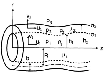
Figure 1: Schematic ofaviscous compound liquid jet.
2
Formulation
Figure 1 shows the schematic of the jet in the $(z, r)$ axisymmetric coordinate system.
Noting that the subscript$j=1$ isrefereed toas thecore phaseorthe inner interface and
$j=2$ as the annular phase or the outer interface, the velocity vectors are denoted by $u_{j}$
whose components
are
$(u_{j}, v_{j})$, while the densities by$\rho_{j}$, theviscosities by $\mu_{j}$, the surface
tensions of the interfaces by $\sigma_{j}$ and the pressures by $p_{j}$. The surfaces are specified at
$r=h_{j}$, while the pressure of the surrounding ambient gas $p_{3}$ is constant and thedensity
is ignored. For convenience of the later analysis, the thickness ofthe annular phase $b$
$(=h_{2}-h_{1})$ and the radius of the mid-plane of the annular phase $R(=(h_{2}+h_{1})/2)$ are
introduced.
In the analysis, we
assume
that the core and annular phases are incompressible andthe gravitational force is ignored. The basic equations are then given by the continuity
and momentum equations for the core phase $(j=1,0\leq r<h_{1})$ and the annular phase
$(j=2, h_{1}<r<h_{2})$
as
follows:$\frac{\partial u_{j}}{\partial z}+\frac{1}{r}\frac{\partial(rv_{j})}{\partial r}=0$,
(1)
$\rho_{j}(\frac{\partial u_{j}}{\partial t}+u_{j}\frac{\partial u_{j}}{\partialz}+v_{j}\frac{\partial u_{j}}{\partial r})=-\frac{\partial p_{j}}{\partial z}+\frac{1}{r}\frac{\partial}{\partial r}[\mu_{j}r(\frac{\partial v_{j}}{\partial z}+\frac{\partial u_{j}}{\partial r})]+\frac{\partial}{\partial z}(2\mu_{j}\frac{\partial u_{j}}{\partial z})$
, (2)
$\rho_{j}(\frac{\partial v_{j}}{\partial t}+u_{j^{\frac{\partial v_{j}}{\partial z}}}+v_{j}\frac{\partial v_{j}}{\partial r})=-\frac{\partial p_{j}}{\partial r}+\frac{1}{r}\frac{\partial}{\partial r}(2\mu j^{r\frac{\partial v_{j}}{\partial r})}+\frac{\partial}{\partial z}[\mu_{j}(\frac{\partial v_{j}}{\partial z}+\frac{\partial u_{j}}{\partial r})]-2\mu_{j^{\frac{v_{j}}{r^{2}}}}.$
(3)
On the other hand, the boundary conditions are given as the kinematical conditions
$\frac{\partial h_{1}}{\partial t}=v_{1}-u_{1}\frac{\partial h_{1}}{\partial z}=v_{2}-u_{2}\frac{\partial h_{1}}{\partial z},$
$u_{1}=u_{2}$ on $r=h_{1}$, (4a)
and the dynamical conditions
$p_{1}=p_{2}+(D_{1}n_{1})\cdot n_{1}-(D_{2}n_{1})\cdot n_{1}+\sigma_{1}\kappa_{1}$and $(D_{1}n_{1})\cdot t_{1}=(D_{2}n_{1})\cdot t_{1}$ on $r=h_{1},$
(5a)
$p_{2}=p_{3}+(D_{2}n_{2})\cdot n_{2}+\sigma_{2}\kappa_{2}$ and $(D_{2}n_{2})\cdot t_{2}=0$ on $r=h_{2}.$
(5b)
In the above representations,
$n_{j}= \frac{(-\partial h_{j}/\partial z,1)}{[1+(\partial h_{j}/\partial z)^{2}]^{1/2}}$ and $t_{j}= \frac{(1,\partial h_{j}/\partial z)}{[1+(\partial h_{j}/\partial z)^{2}]^{1/2}},$
are, respectively, the normal and tangential vectors and
$D_{j}=\mu_{j}\{\begin{array}{ll}2\partial u_{j}/\partial z (\partial v_{j}/\partial z+\partial u_{j}/\partial r)(\partial v_{j}/\partial z+\partial u_{j}/\partial r) 2\partial v_{j}/\partialr\end{array}\},$
aretheviscous stresstensors, whilethe surface tensions$\sigma_{1}\kappa_{1}$ and$\sigma_{2}\kappa_{2}$ act onthe surfaces
when the curvatures
are
givenas
$\kappa_{j}=\frac{1}{h_{j}[1+(\partial h_{j}/\partial z)^{2}]^{1/2}}-\frac{\partial^{2}h_{j}/\partial z^{2}}{[1+(\partial h_{j}/\partial z)^{2}]^{3/2}}.$
Thenon-Newtonian viscosity is presented by the following Carreau model [8]:
$\mu_{j}=\mu_{0j}M_{j}$ and $M_{j}=[1+(\alpha\dot{\gamma}_{j})^{2}]^{(n-1)/2}$ (6)
where $\mu_{j}$ arethe apparent viscosities and $\dot{\gamma}_{j}$ arethe deformation rates whichare given as
the second invariant in terms of$u_{j}$ and $v_{j}$ in the followingforms $(j=1,2)$:
$\dot{\gamma}_{j}=\sqrt{2(\frac{\partial v_{j}}{\partial r})^{2}+2(\frac{v_{j}}{r})^{2}+(\frac{\partial v_{j}}{\partial z}+\frac{\partial u_{j}}{\partial r})^{2}+2(\frac{\partial u_{j}}{\partial z})^{2}}.$
In the representations of (6), the time constant $\alpha$ takes about 1 to 10 depending upon
materials, while the power low exponent $n(>0)$ takes less than 1 when the viscosity is
pseudo-plasticand larger than 1 when dilatant and unity when Newtonian.
The basic equations and the boundary conditions
can
be simplified by using the longwave
approximation in which sufficiently long waves are considered compared with thecoreradius and annular thickness. In thepresentanalysis,weintroduce theapproximation
withdifferent expansion parameters to thecoreand the annularphases. Then, we
assume
the variables of the core phase to be expanded in terms of$r^{2}$ due to the axisymmetry at
$r=0$, while the annular phasein terms of$r-R$
as
follows:$u_{1}=u_{1}^{(0)}+r^{2}u_{1}^{(2)}+\cdots, p_{1}=p_{1}^{(0)}+r^{2}p_{1}^{(2)}+\cdots,$
$u_{2}=u_{2}^{(0)}+(r-R)u_{2}^{(1)}+(r-R)^{2}u_{2}^{(2)}+\cdots,$
$v_{2}=v_{2}^{(0)}+(r-R)v_{2}^{(1)}+(r-R)^{2}v_{2}^{(2)}+\cdots$ , (7)
where the coefficients
are
functions of$z$ and $t$. The jet equations arederived in a similarway to the Newtonian viscous case [7]. Using the above expansions (7) int$0$ the basic
equations and the boundary conditions (1)$-(5)$ and the representations of the viscosity
(6), and neglecting the higher order terms than $O(h_{1})$ and $O(b)$, we finally obtain the
following reduced equations for $b,$ $R,$ $u_{1},$ $u_{2},$ $v_{2}$ in the lowest order of the approximation
(superscripts on the variables have been omitted):
$\frac{\partial b}{\partial t}=-\frac{\partial(bu_{2})}{\partial z}-\frac{bv_{2}}{R}$,
(8a)
$\partial R \partial R$
$\overline{\partial t}\overline{\partial z}=v_{2}-u_{2}$, (8b)
$\frac{\partial u_{1}}{\partial t}=-u_{1}\frac{\partial u_{1}}{\partial z}-\frac{1}{\rho}\frac{\partial p_{1}}{\partial z}+\frac{\mu}{\rho{\rm Re}}(M_{1}f_{11}+\frac{\partial M_{1}}{\partial z}f_{12})$ , (8c) $\frac{\partial u_{2}}{\partial t}=-u_{2}\frac{\partial u_{2}}{\partial z}-(\frac{\partial P}{\partial z}-\frac{\triangle P}{b}\frac{\partial R}{\partial z})+\frac{\mu}{{\rm Re}}(M_{1}f_{21}+\frac{\partial M_{1}}{\partial r}f_{22})$
$+ \frac{1}{{\rm Re}}(M_{2}f_{23}+\frac{\partial M_{2}}{\partial r}f_{24}+\frac{\partial M_{2}}{\partial z}f_{25})$ ,
(8d)
$\frac{\partial v_{2}}{\partial t}=-u_{2}\frac{\partial v_{2}}{\partial z}-\frac{\triangle P}{b}+\frac{\mu}{{\rm Re}}M_{1}f_{31}+\frac{1}{{\rm Re}}(M_{2}f_{32}+\frac{\partial M_{2}}{\partial r}f_{33}+\frac{\partial M_{2}}{\partial z}f_{34})$, (8e)
together with the equation for$p_{1}$ to connect the motions of the
core
and annular phases$A_{1} \frac{\partial^{2}p_{1}}{\partial z^{2}}+A_{2}\frac{\partial p_{1}}{\partial z}+A_{3}p_{1}+A_{4}=0$. (8f)
In the above representations,
$P = \frac{1}{2}(p_{1}+p_{3})-\frac{1}{2Wb}(\sigma\kappa_{1}-\kappa_{2}) , \triangle P =-(p_{1}-p_{3})+\frac{1}{Wb}(\sigma\kappa_{1}+\kappa_{2})$,
are, respectively, like a mean pressure and a pressure difference of $p_{1}$ and $p_{3}(=const.)$
when the surface tension is taken int$0$ account. The above set of equations have been
normalized in terms of a characteristic length $H$, speed $U$, time $H/U$ and pressure
$\rho_{2}U^{2}$, while the non-dimensional parameters of the Weber number Wb
$=\rho_{2}HU^{2}/\sigma_{2},$
the Reynolds number ${\rm Re}=\rho HU/\mu_{2}$, the density ratio $\rho=\rho_{1}/\rho_{2}$, the viscosity ratio
$\mu=\mu_{01}/\mu_{02}$ and the surfacetension ratio $\sigma=\sigma_{1}/\sigma_{2}$ areintroduced based on the annular
phase. We can show that the viscous terms $f_{ij}(i=1,2,3, j=1,2, \cdots)$ in Eqs.(8c) to
(8e) are functions of$b,$$R,$$u_{1},$ $u_{2},$$v_{2}$, while the coefficients $A_{1}$ to $A_{4}$ in (8f) are functions
of $b,$$R,$$u_{1},$ $u_{2},$$v_{2}$ including $f_{ij}$ and $\kappa_{j}$ together with $Re,$ $\mu,$ $\sigma$ and
$\rho$. Consequently, the
problem can be reduced tosolving the above simplified nonlinearequations (8a) to (8f).
In particular, for an infinitely long jet on the steady state without any velocity
dif-ference betweenthe
core
and annular phases, we take the radii and flow velocities to be constant such as $h_{1}=\overline{h}_{1},$ $h_{2}=\overline{h}_{2},$ $u_{1}=\overline{u}_{1}=u_{2}=\overline{u}_{2},\overline{v}_{1}=\overline{v}_{2}=0$. Then, we canset $f_{ij}=0$ and $\triangle P=0$, from which $\overline{p}_{1}$ is found to be always larger than
$p_{3}$ due to the
surface tension
where $\overline{R}=(\overline{h}_{1}+\overline{h}_{2})/2,$ $\overline{b}=\overline{h}_{2}-\overline{h}_{1}.$
Next
we are
going to numerically examine initial-boundaryvalue problems fordistur-bances superimposedonthe above steady state, where the characteristic values
are
chosenas $H=\overline{h}_{2}$ and $U=\overline{u}_{2}.$
3
Numerical Results
Numerical calculations
are
carried out bymeans
of the 4th order Runge-Kutta methodfor the timederivatives and the finitedifference method for the spatialderivatives, where the$3rd$-order upwinding scheme is used for the convective terms and the central difference
method whose error is of$O(\Delta z^{2})$ is used for the otherspatial derivatives. The numerical
time and spatial grid sizes $\Delta t$ and $\triangle z$ are, respectively, taken to be 0.05 and 0.2 for
most of the calculations, for which sufficient numerical accuracy is retained with respect
to the volumes of the
core
and annular phases. We consider the initial-boundary valueproblems that the jet is in the steady state whose pressure difference is given by Eq.(9)
for $0\leq z<\infty$ when $t=0$, while the velocity disturbances
$u_{1}-1=u_{2}-1=\eta\sin(\omega t)$, (10) are applied to the nozzle exit at $z=0$ for $t>0$. In the calculations, the amplitude of
disturbance$\eta$is taken to be0.005 andthe domain region of$z$forthecalculations istaken
to be enough large comparing with the breakupdistance $z_{b}$ (in most of the cases, $z=200$
to 300).
In the analysis, we examine the breakup time $t_{b}$ and distance $z_{b}$ for various input
frequency$\omega$, where we decide the breakup when the core radius or the annular thickness
becomes sufficiently small to the extent of0.001. Resulting from this, we
can
determinethe critical frequencies $\omega_{c}$ which minimize $t_{b}$ for each parameters Wb, $Re$, and
$\sigma$
.
Suchfrequencies $\omega_{c}$
are
the most unstable input frequencies in thesense
of nonlinearity andcanwell predict the natural formation periods of capsules [6]. This is expected to be still valid in the preset
case.
In the following, unless noted otherwise, we take $\rho=1,$ $\mu=1,$ $\overline{u}_{1}=\overline{u}_{2}=1,\overline{h}_{1}=0.485$ and $\overline{h}_{2}=1$as
the basic parameters according to the experimentforthe liquid-cored jet by Hertz andHermanrud [4]. All of the presented results
are
those at $\omega_{c}$ resulting from carrying out the calculations forvarious input$\omega$ from 0.2 to 1.6 for
each parameters. In addition,
we
take $\alpha=0.5$and$n=0.2$ and1.8
for the non-Newtonianviscosities, while $n=1$ for the Newtonianviscosity in Eq.(6).
First, we consider the weak viscous case of${\rm Re}=395$and Wb $=47.9$ whose values are
of the experiment [4]. Figure 2 for sufficiently small $\sigma=0.1$ shows that the jet breaks
up like a single phase column jet where the core phase pinches by closing the annular
phase, which is expected to produce a train of liquid capsules. On the other hand, Fig.3
for larger $\sigma=2.6$ shows that the core phase becomes unstable to be pinched prior to
theannular phase because oflarger surface tension ratio, which is expected to produce
a
train ofcore liquid drops in the sheath of annular phase and delaythe the annular phase
instability. We note that these breakup profiles are closely similar to the experimental
results [4]. However, for different values of $n$ , we cannot find any salient discrepancies
(a) (a) $z$ $z$ (b) (b) $z$ $z$ (c) (c) $z$ $z$
Figure 2: Breakup profiles for different $n$ Figure 3: Breakup profiles for different
when $\sigma=0.1,$ ${\rm Re}=354$ and Wb $=47.9$ $n$ when $\sigma=2.6,$ ${\rm Re}=354$ and Wb $=$
$;(a)n=0.2(t_{b}=85.90, z_{b}=80.60, \omega_{c}= 47.9;(a)n=0.2(t_{b}=28.75,$ $z_{b}=25.80,$
0.80), $(b)n=1(t_{b}=85.95, z_{b}=80.60, \omega_{c} = 1.35),$ $(b)n$ $=$ 1 ($t_{b}$ $=$ 28.75,
$\omega_{c}=0.80)$ and $(c)n=1.8(t_{b}=85.95, z_{b}=25.80, \omega_{c}=1.35)$ and $(c)n=1.8$
$z_{b}=80.60,$ $\omega_{c}=0.78)$. $(t_{b}=28.80, z_{b}=25.80, \omega_{c}=1.35)$.
critical frequency $\omega_{c}$ among (a), (b) and (c) in each Figs.2 and 3, where $(a)t_{b}=85.90,$
$z_{b}=80.60,$ $\omega_{c}=0.80,$ $(b)t_{b}=85.95,$ $z_{b}=80.60,$ $\omega_{c}=0.80$ and $(c)t_{b}=85.95,$ $z_{b}=80.60$
and $\omega_{c}=0.78$ in Fig.2, while $(a)t_{b}=28.75,$ $z_{b}=25.80,$ $\omega_{c}=1.35,$ $(b)t_{b}=28.75,$
$z_{b}=25.80,$ $\omega_{c}=1.35$and $(c)t_{b}=28.80,$ $z_{b}=25.80,$ $\omega_{c}=1.35$ in Fig.3. This shows that
the non-Newtonianviscosity does not affect the breakup properties when the viscosity is
weak or large $Re.$
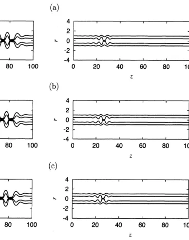
Nextweconsider themoreviscouscaseof${\rm Re}=10$. Figure4 for$\sigma=0.1$shows that the
non-Newtonian viscosity does not still affect the breakup properties such
as
the breakuptime anddistanceandcriticalfrequencyaswellasthe breakup profiles among(a), (b) and (c), where $(a)t_{b}=211.15,$ $z_{b}=200.80,$ $\omega_{c}=0.50,$ $(b)t_{b}=205.50,$ $z_{b}=200.80,$ $\omega_{c}=0.50$
and $(c)t_{b}=205.55,$ $z_{b}=200.80$ and $\omega_{c}=0.50$. We note that $t_{b}$ and $z_{b}$ increase and $\omega_{c}$
decreases as the decrease of ${\rm Re}$ in comparison between Fig.2 and Fig.4. However, Fig.5
$n$. In the Figure,
we
find that the jet shows the typical three different breakups, thatis, disintegration of the annular phase for$n=0.2$ and the large ballooned annular phase
when $n=1$ and the closing of the annular phase with pinching the core phase when
$n=1.8$
.
In spite of the fact that the breakup profiles and $\omega_{c}$are
different for $n$, there islittle discrepancy in the breakup time and distance, where $(a)t_{b}=111.95,$ $z_{b}=109.40,$
$\omega_{c}=0.72,$ $(b)t_{b}=122.20,$ $z_{b}=120.00,$ $\omega_{c}=0.58$ and $(c)t_{b}=125.80,$ $z_{b}=120.60,$
$\omega_{c}=0.40$. This means that thedeformations of thejet areaccelerated rapidly onlynear
thebreakup. Asaresult, thenon-Newtonian viscosity may bring about these three types
of breakup depending upon the values of $n$ when ${\rm Re}$ is small and $\sigma$ is not sufficiently
small.
Since the breakupdue to closing of the
core
phase ispreferable for encapsulation andthe disintegration or ballooning of the annular phase should be avoided for successful
capsule producing, it is worth to reveal what types of the breakup tend to appear in the
parameter region of Wb and $\sigma$. In Fig.6weshow theclassification of the breakup profiles
in the parameter regionsfor $n=0.2,1$ and 1.8 when ${\rm Re}=10$, where the symbols $\triangle,$
and $\bullet$ denote that the breakup is caused by the disintegration, ballooning and closing,
respectively, corresponding to (a), (b) and (c) in Fig.5. We
can
find from Fig.6(a) for$n=0.2$, the breakup is almost due to disintegration except for small $\sigma$
.
On the otherhand, from Fig.6(b) for$n=1$ the parameter region of closing increases and the region of
disintegrationis replaced by the ballooning, where the disintegration without ballooning
isplaced in between the closingand ballooningin most ofthe cases, though the breakup
by the ballooning is finally caused by disintegration of the annular phase. However, we
find in Fig.6(c) for $n=1.8$ that the region ofthe disintegration disappears and the region
ofclosing more increases. These characteristic breakup profiles for different $n$ show that
the breakup isoften caused by disintegration when theviscosity decreases asthe increase
of the deformation rate$\dot{\gamma}(n<1)$, while thebreakupis often byclosingwhen the viscosity
increases as the increase of$\dot{\gamma}(n>1)$.
Inspiteof these three distinctbreakup profilesfor different$n$,
we
cannot findso
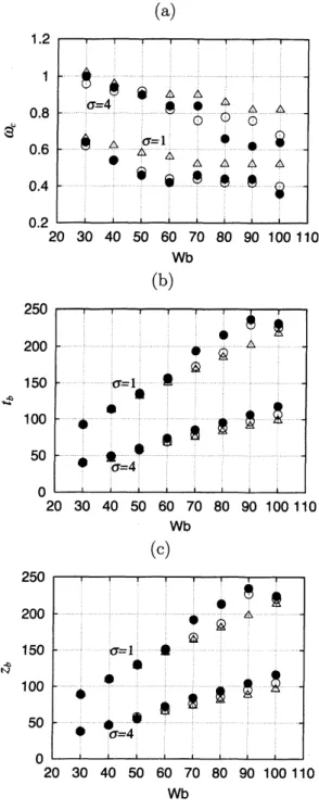
evidentdiscrepancies in the breakup time and distance. This is shown in Fig.7, where variations
of$\omega_{c},$ $t_{b}$ and $z_{b}$ are presented in (a), (b) and (c) when Wb and $\sigma$ ($=1$ and 4)
are
given,in each of which the cases of$n=0.2,1$ and 1.8 are, respectively, denoted by $\triangle,$
$\bullet$. It is found from the Figure that the values of$t_{b}$ and $z_{b}$ for different $n$ agree well with
each other unlessWb issolarge, though$\omega_{c}$ arerather different for$n$. Thismeansthat the
effects of the non-Newtonian viscosity appear only
near
the breakup since the breakuptime anddistance
are
little affected by $n$even
if the breakup profilesare
rather different. Since most of the polymer liquids for the practicaluse are
pseudo-plastic $(n<1)$,the jet is apt to break up by disintegration of the annular phase at the encapsulation
for low $Re$. Therefore, we need to set suitable experimental condition and choose proper
materials for successful capsule formation.
4
Conclusions
By using the long wave approximation we have derived the nonlinear equations of the
the most unstable input frequencies when sinusoidal disturbances are fed at the nozzle exit ofthesemi-infinitejet, the following conclusions are obtained :
1. For larger Reynolds numbers $Re$, the jet breaks up like a single phase column jet
when$\sigma$issufficientlysmall, while thecorephase breaks up by pinching before closing
of the annular phase for larger $\sigma$
.
Any influence of the non-Newtonian viscosity onthe breakup propertiesis not observed for different values of$n.$
2. For smaller $Re$, the jet still breaks up like a single phase column jet
as
long as $\sigma$is sufficientlysmall. The non-Newtonian viscosity also does not affect the breakup
properties for different values of$n.$
3. When$\sigma$ becomes large for small $Re$, however, the breakup profilesbecome different
dependingupon$n$in thenon-Newtonian viscosity. For smaller$n(<1)$, the jet tends
to break up by disintegration of the annular phase, while the breakup for larger $n$
$(>1)$ mainlyresultsfrom the ballooning orclosingof the annular phase. Generally,
as the increase of$n$, the breakup by closing of the annular phase is more dominant
in the Wb and $\sigma$ parameter region.
4. Theinfluence ofthe non-Newtonian viscosityon$t_{b}$ and $z_{b}$ is not
so
largeeven
whensmall${\rm Re}$andlarge$\sigma$. Thismeansthat theeffect ofnon-Newtonian viscosityappears
only
near
the breakup of the jet.5. Thejet usingpolymer liquids for small${\rm Re}$ is apt tobesubject tothe annularphase
disintegration, which prevents the successful encapsulation.
Acknowledgment
This work has beenpartially supported bytheGrant-in-Aid forScience Research from the
Ministry of Education, Culture, Sports, Science and Technology ofJapan (No.21560177).
References
[1] Lefebvre,A.$H$., Atomization andsprays (Hemisphere, New York, 1989).
[2] Lin,S.$P$., Breakup
of
liquid sheets andjets (Cambridge, 2003).[3] Kendall,J.$M$., Phys. Fluids 29, 2086-2094 (1986).
[4] Hertz, C.$H$. and Hermanrud, B., J. Fluid Mech. 131, 271-287 (1983).
[5] Yoshinaga,T. and Maeda,M., J. FluidScience and Technology 4, 324-334 (2009).
[6] Yoshinaga,T.,ICLASS 2009, Colorado, USA July 26-30, 2009.
[7] Yoshinaga,$T$ and Yamamoto,K., J. Fluid Science and Technology 6, 477-486 (2011).
(a) (a) $z$ $z$ (b) (b) $z$ $z$ (c) (c) $z$ $z$
Figure 4: Breakup profiles for different $n$
Figure 5: TyPical three breaku$P$
profiles-when $\sigma=0.1,$ ${\rm Re}=10$ and Wb $=47.9$:
disintegration, ballooning and closing- for
$(a)n=0.2(t_{b}=211.15,$ $z_{b}=200.80,$ $\omega_{c}=$
different $n$ when $\sigma=2.6,$ ${\rm Re}=10$ and
0.50), $(b)n=1(t_{b}=205.50,$ $z_{b}=200.80,$ $\sim$ げ $=80;(a)n=0.2(t_{b}=111.95,$ $z_{b}=$ $\omega_{c}=0.50)$ and $(c)n=1.8(t_{b}=205.55,$ 109.40, $\omega_{c}=0.72),$ $(b)n=1(t_{b}=122.20,$ $z_{b}=200.80,$ $\omega_{c}=0.50)$. $z_{b}=120.00,$ $\omega_{c}=0.58)$ and $(c)n=1.8$ $(t_{b}=125.80, z_{b}=120.60, \omega_{c}=0.40)$.
(a) (a) Wb Wb $($b$)$ $($b$)$ Wb Wb $($c$)$ $($c$)$ Wb Wb
Figure 6: Classificationsof the breakup $prx$ Figure 7: Variations of$\omega_{c},$ $t_{b}$ and $z_{b}$ for Wb
files in the parameter space Wb and $\sigma$ when when$\sigma=1$ and4and${\rm Re}=10$,where$\triangle:n=$
${\rm Re}=10$, where $\triangle,$
denote the cases when the breakup is due to
disintegration, ballooning and closing of the
annular phase: $(a)n=0.2,$ $(b)n=1$ and