Positive solutions to some cross-diffusion systems in population dynamics (Dynamics of spatio - temporal patterns for the system of reaction - diffusion equations)

Positive

solutions

to

some

cross-diffusion

systems

in population dynamics

Kousuke KUTO

(

久藤衡介

)*

Department of

Mathematics,

Waseda University

3-4-1

Ohkubo,

Shinjuku-ku,

Tokyo,

169-8555

JAPAN

1Introduction

In thisarticle, we

are

concerned withthefollowing strongly coupled parabolic

sys-$\mathrm{t}\mathrm{e}\mathrm{m}$;

(P)$\{$

$u,$ $=\Delta[(1+\alpha v)u]+u(a-u -cv)$ in $\Omega\cross(0, T)$,

$v_{t}= \Delta[(\mu+\frac{1}{1+\beta u})U]$ $+v(b+du -v)$ in $\Omega\cross(0, T)$,

$u=u$ $=0$ on

an

$\cross(0, T)$,

$u(\cdot, t)=u_{0}\geq 0$_, $v( \cdot, t)=v_{0}\geq 0$ on $\Omega$,

where $\Omega$ is abounded domain in $R^{N}$ withasmooth boundary

an;

$a$,$b$,$c,d$ and$\mu$ are

all positive constants; $\alpha$and$\beta$ are nonnegativeconstants. System (P) is one of

Lotka-Volterraprey-predator models with nonlineardiffusion effects. From such

an

ecologi-cal model point ofview, unknown functions $u$ and$v$represent population densities of

prey and predator, respectively. In reactionterms, $a$ and$b$

are

birth rates ofrespective

species, $c$ and $d$ mean prey-predator interactions. In the first equation, the nonlinear

diffusion term$\mathrm{a}\mathrm{A}(\mathrm{u}\mathrm{v})$ describes atendencysuch that the

prey

specieskeep

away

from

high density

areas

ofthepredator species. This term $\mathrm{a}\mathrm{A}(\mathrm{u}\mathrm{v})$ is usually referred

as

the

cross-diffitsion

term. Acompetition population model withcross-diffusion terms

was

firstproposedby Shigesada-Kawasaki-Teramoto [29]. Sincetheirpioneerwork,many

mathematicianshavediscussed population models withcross-diffusiontermsfrom

var-ious view points,

e.g.,

theglobal existence oftime-depending solutions ([1], [3], [81,

[9], [10], [24], [301) and steady-stateproblems ([13], [14], [16], [21], [22], [23], [25], [26], [28]$)$. In thesecondequation,thefractionaltype nonlineardiffusion$\Delta(\frac{v}{1+\beta u})$

mod-elsasituation such that thepopulation

pressure

of thepredatorspeciesweakens in high

$*\mathrm{e}$-mail address: kuto$toki was $\mathrm{e}\mathrm{d}\mathrm{a}$.

density

areas

of the

prey

species. To my knowledge, there arefew works about such

fractionaltypenonlinear$\mathrm{d}\mathrm{i}\mathrm{f}\mathrm{f}\mathrm{i}\mathrm{s}\mathrm{l}\mathrm{o}\mathrm{n}|$

effectsin

a

field ofreaction-diffision systems.

Inthepresentarticle,

we

will mainly discussthe associate steady state problem;

(SP) $\{$

$\Delta[(1+\mathrm{a}\mathrm{v})\mathrm{u}]$ $+u(a-u-cv)$ $=0$ in $\Omega$, $\Delta[(\mu+\frac{1}{1+\beta u})v]$$+v(b+du-v)$ $=0$ in $\Omega$,

$u=v=0$ on $\partial\Omega$.

Amongother things,

we

are

interestedin positivesolutions of(SP).Fromtheview point

of theprey-predatormodel,

a

positive solution $(u,v)$

means

a coexistence steady state.

So it is importantto study thepositive solution set of(SP). Ourfirst aimis to obtain

a

sufficientcondition ofcoefficients $(\alpha,\beta,\mu, a, b, c, d)$for existence ofpositive solutions

to (SP). Our approachto theproof is based

on

the bifurcationarguments. Throughout

the article,

we

$\mathrm{w}\mathrm{i}\mathrm{U}$ regard the coefficient

$a$ $\mathrm{a}_{\mathrm{c}}^{\epsilon}\mathrm{i}$ a positive bifurcation parameter. Our

strategyis to seek

a

bifurcation point

on

the semitrivial solution setsby making useof

the local bifurcation theory ([4]). Here

a

semitrivial solution

means a

solution $(n, v)$

such that either$u$or$v$vanishesin$\Omega$. We willfind

a

certainnumber

$a^{*}=a^{*}(\alpha,\mu, b, c, d)$

suchthatpositivesolutionsbifurcate from the semitrivial solution with $u$ $\equiv 0$ at_$a=a^{*}$.

if$b>(\mu+1)\mathrm{A}\mathrm{i}$, where $\lambda_{1}$ is denoted by the leasteigenvalue $\mathrm{o}\mathrm{f}-\Delta$with the

homoge-means

Dirichlet boundary condition on $\partial\Omega$. On the other hand, if _{$b<(\mu+1)\mathrm{A}\mathrm{i}$}, we

will get

a

certain $a_{*}=a_{*}(\beta,\mu, b, c, d)$ such that positive solutions bifurcate from the

semitrivial solution with$v$ $\equiv 0$ at_{$a=a_{*}$}

.

By

a

combination with the globalbifurcation

theory ([27]) and

some

apriori estimates forpositive solutions, we willprove that the

positive solutionbranchbifurcates from

a

semitrivial solution at$a=a^{*}$ or$a=a_{*}$ and

extends globally with respect to $a$

.

Therefore, we know that (SP) admits at least one

positive solutionif$b>(\mu+1)\lambda_{1}$ (resp.$b<(\mu+1)\lambda_{1}$) and$a>a^{*}$ (resp.$a>a_{*}$).

Our second aim is to derive a large nonlinear diffision effect of$\beta$ on the positive

solution setto (SP) with a

case

when $\alpha=0$ and $b>(\mu+1)\lambda_{1}$. Forthe sake of this

derivation, we will introduce two shadow systems

as

$\betaarrow\infty$ in (SP) with $\alpha=0$. Let

$\{\beta_{n}\}$beanysequencewith

$\lim_{narrow\infty}\beta_{n}=\infty$and

suppose

that{(un,$u_{n}$)} isanypositivesolution

sequence

to (SP) with $\alpha=0$and$\beta=\beta_{n}$. Under

some

additionalassumptions, wewill

prove

thatsubjectto

a

subsequence,

one

of thefollowingtwo

cases

necessarilyoccurs:

(i) Thereexists

a

certainpositive solution$(u, v)$ of

$\{$

$\Delta u+u(a-u-cu)=0$ in $\Omega$, $\mu\Delta v$ $+v(b+du-v)$ $=0$ in $\Omega$,

$u=u=0$ on $\partial\Omega$,

(1.1)

such that$\lim_{narrow\infty}(u_{n},v_{n})=(u, v)$ in

(ii) Thereexists

a

certain positive solution$(w, v)$ of

$\{$

$\Delta w+w(a-cu)=0$ in $\Omega$,

$\Delta[(\mu+\frac{1}{1+w})v]+v(b-v)=0$ in $\Omega$,

$w=v=0$ on $\partial\Omega$,

(1.2)

such that$\lim_{n\prec\infty}(\beta_{n}u_{n}, \iota)_{n})=(w, v)$ in

$L^{\infty}(\Omega)^{2}$.

Our

convergence

result (Theorem 3.1) $\mathrm{w}\mathrm{i}\mathrm{U}$ also assert that if$\beta$ is sufficiently large,

any positive solution of(SP) (with $\alpha$ $=0$)

can

be approximated by

a

certain positive

solution of either (1.1) or (1.2). So it is natural to ask which of(1.1) or (1.2) (or both)

cancharacterizepositive solutions of(SP),ineach coefficient$(lr, a, b, c, d)$

case.

There

are many studies about the first shadow system (1.1) (see

e.g.,

[2], [5], [6], [7], [17],

[18], [19], [20], [31]$)$. According to thelr results, for any $(\mu, b, c, d)$ fixed,

we

have a

thresholdnumber\^a$(>a^{*})$ such that(1.1)admitsa positivesolutionifand onlyifa>\^a.

Thus it is

a

cmcial part ofthis article to study the positive solution set of the second

shadow system(1.2). By regarding $a$

as a

bifurcationparameter,

we

will showthatthe

branch of the positive solution set of(1.2) bifurcates from

a

semitrivial solution with

$w\equiv 0$ at $a=a^{*}$, and extends globally with respect to $w$

.

(The branch is unifomly

bounded withrespectto $(v, a).)$ Furthemore,

we

will

prove

that the branch necessarily

blows

up

with respectto$||w||_{\infty}$ ata=\^a. Sothisresult also impliesthatpositive solution

set of(SP) (with $\alpha=0$) stmcturally changes

near

a=\^a, when$\beta$ is sufficiently large

(Theorem 3.8).

ThroughouttheaHicle,

we

willdenoteby$\lambda_{1}(q)$the least eigenvalue of theproblem

$-\Delta u+q\{x$)$u$ $=\lambda u$ in $\Omega$, $u=0$ on $\partial\Omega$,

where $q(x)|1\mathrm{S}$

a

continuous function in

$\overline{\Omega}$

. We simply write $\lambda_{1}$ instead of $\lambda_{1}(0)$

.

Itis

well knownthatthefollowingproblem

$\Delta u+u(a-u)=0$ in $\Omega$, $u=0$

on

$\partial\Omega$ (1.3)

has aunique positive solution$u=\theta_{a}$ ifand onlyif$a>\lambda_{1}$. Then (SP) has

a

semitrivial

solution$(\mathrm{w}, v)$ $=(\theta_{o}, 0)$if$a>\lambda_{1}$. Furthemore it is easily verllfied that(SP) has another

semitrivial solution $(u, v)=(0, (\mu+1)\theta_{b/(\mu+1)})$ if$b>(\mu+1)\lambda_{1}$. Here, $\theta_{b/(lx+1)}$ represents

a

positivesolution of(1.3)with$a$replaced by$b/(\mu+1)$

.

The usual

noms

of the

spaces

$L^{p}(\Omega)$ for$p\in[1, \infty)$ and$C(\overline{\Omega})$

are

definedby

$||u||_{p}:=( \int_{\Omega}|u(x)|^{p}dx)^{1/p}$ and

$||u||_{\infty}:= \mathrm{m}_{X\in}\mathrm{x}\frac{\mathrm{a}}{\Omega}|u(x)|$

.

The contents of the present article

are

as

follows: In Section 2, we first give the

sufficientcondition forexistenceofpositive solutionsto(SP).Next

we

givetheoutline

of the proof. In Section 3, we will discuss a special casewhen$\beta$ is sufficiently large.

The above convergence to one oftwo shadow systems as$\betaarrow\infty$ will be justified in

this section. The solution set of(1.2) willbe studilled inthe latter half of thissection.

2

Coexistence

Region

2.1

Main Result

In this section,

we

firstgive

a

sufficient conditionofexistence ofpositive solutions

to (SP).

Theorem

2.1.

_If

$a\leq\lambda_{1}$, then (SP) has

no

positive solution. In

a case

when $a>\lambda_{1}$,

(SP) admits

a

positive solution

_if

the$fo$llowing condition (2.1)holds true.

$\lambda_{1}(\frac{c(\mu+1)\theta_{b/(\mu+1)}-a}{1+\alpha(\mu+1)\theta_{b/(\mu+1)}})<0$ and $\lambda_{1}(-\frac{(b+d\theta_{a})(1+\beta\theta_{a})}{\mu(1+\beta\theta_{a})+1})<0$

.

(2.1)

Here it is

_defined

that$\theta_{b/(u+1)}\equiv 0$

if

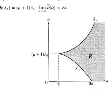
$b\leq(\mu+1)\lambda_{1}$.

We need to explain the meaning ofTheorem 2.1. Regarding $a$ and $b$ as positive

parameters, weintroducethefollowing two sets inthe $(a, b)$plane,

$S_{1}:=\{(a, b)\in R_{+}^{2}$

:

$\lambda_{1}(-\frac{(b+d\theta_{a})(1+\beta\theta_{a})}{\mu(1+\beta\theta_{a})+1})=0$ for $a\geq\lambda_{1}\}$ .

$S_{2}:=\{(a, b)\in R_{+}^{2}$ : $\lambda_{1}(\frac{c(\mu+1)\theta_{b/(\mu+1)}-a}{1+\alpha \mathrm{Q}x+1)\theta_{b/(\mu+1)}})=0$ for _{$b\geq(\mu+1)\lambda_{1}\}$}.

The following Lemmas 2.2 and 2.3 mention the shapes of

curves

$S_{1}$ and $S_{2}$,

respec-tively. See [12] forthe proofs ofLemmas2.2 and2.3.

Lemma

2.2.

There exists

a

certain$a_{0}>\lambda_{1}$ such that$S_{1}$ can beexpressed

as

$S_{1}=$ $\{(a, b)\in R_{+}^{2} : b=\mathrm{b}(\mathrm{a}) for \lambda_{1}\leq a<a_{0}\}$_,

where $b=\mathrm{b}(\mathrm{a})$ is

a

positive continuous

function

_$for$ $a\in[\lambda_{1}, a_{0})$, and

satisfies

the

$fo$llowingproperties :

(i) $\underline{b}(\lambda_{1})=(\mu+1)\lambda_{1},\lim_{aarrow a_{0}}\underline{b}(a)=0$.

Lemma2,3. _Theset$S_{2}$possessesthe expression

$S_{2}=$ $\{(a, b)\in R_{+}^{2} : b=\overline{b}(a) for a\geq\lambda_{1}\}$,

where $b=\overline{b}(a)$ is

a

positive continuous

function

$for$ $a\in[\lambda_{1}, \infty)$, and

satisfies

the

followingproperties :

(i) $\overline{b}(a)$ isamonotone increasingfunction withrespectto $a$.

$(1 \mathrm{i})\overline{b}(\lambda_{1})=(\mu+1)\lambda_{1},\lim_{aarrow\infty}\overline{b}(a)=\infty$.

Fig.1 : Coexistence Region

Combining theseproperties of$S_{1}$ and$S_{2}$,one candeduce from Theorem2.1 that if

$(a, b)$lies in aregion$R$ surrounded by$S_{1}$ and 52, then (SP) hasa positivesolution (see

Fig. 1). This$R$, in case$\alpha=\beta$ $=0$, correspondsto theexactcoexistence region shown

by $\mathrm{L}\acute{\mathrm{o}}\mathrm{p}\mathrm{e}\mathrm{z}_{\lrcorner}$-G\’omezand Pardo [19]. Fromaview-point of thebifurcation theory,

we

will

prove

thatpositivesolutionsbifurcatefrom$(u, v)$ $=(\theta_{a}, 0)$when$(a, b)$

crosses

$S_{1}$ curve.

Similarly positive solutions also bifurcate from $(u, v)$ $=(0, (\mu+1)\theta_{b/(\mu+1)})$when $(a,b)$

moves

across

$S_{2}$.

2.2

Apriori Estimates

In therestpart of the section, we givethe outline ofthe proofofTheorem 2.1. In

this subsection, wefirstintroduce a semilinear elliptic system equivalentto (SP), and

next give some apriori estimates ofpositive solutions to the semilinear system. Such apriori estimates $\mathrm{w}\mathrm{i}\mathrm{U}$make an importantrules in theproof. Assume $(\alpha,\beta)\neq(0, 0)$in

(SP).As long

as we are

restrictedonnonnegative solutions,it isconvenienttointroduce

twounknown functions $U$ and$V$by

Thereis

a

one-t0-0ne correspondence between$(u, u)\geq 0$ and $(U, V)\geq 0$

.

Itis possible

todescribe their relations by

$u=u(U, V)$

$= \frac{-(\alpha V+1)+\mu(\beta-1)+\sqrt{\{(\alpha V+1)-\mu(\beta-1)\}^{2}+4\beta(\alpha V+\mu)(1+\mu)}}{2\beta(\alpha V+\mu)}$_,

(2.3)

$v$ $=v(U, V)$

$= \frac{\alpha V-1-\mu(\beta U+1)+\sqrt{\{(\alpha V-1)-\mu(\beta U+1)\}^{2}+4\alpha V(\beta U+1)(1+\mu)}}{2\alpha(1+\mu)}$.

Since we are concemedwith nonnegative solutions, (SP) is rewritten in the following

equivalent fom

(BP) $\{$

$\Delta U+u(a-u-cu)$ $=0$ in $\Omega$,

$\Delta V+v(b+du-u)=0$ in $\Omega$ ,

$U=V=0$ on $\partial\Omega$,

where $u=u(U, V)$ and $v$ $=v(U, V)$ are understood

as

functions of $(U, V)$ defined by

(2.3). Itis

easy

toshowthat (EP)hastwo semitrivial solutions

$(U, V)=(\theta_{a}, 0)$ for $a>\lambda_{1}$ and $(U, V)=(0, (\mu+1)^{2}\theta_{b/(\mu+1)})$ for $b>(\mu+1)/\mathrm{i}\mathrm{i}$,

in addition to the trivial solution $(U, V)=(0,0)$

.

We obtain the following apriori

esti-matesforpositive solutions of(EP).

Lemma

2.4.

Suppose that $(U, V)$ is anypositive solution

of

(EP) andthat $(\mathrm{w}, v)$ is any

positive solution

_of

(SP). Then,$for$all$x\in \mathrm{q}$

$0\leq \mathrm{V}(\mathrm{x})\leq \mathrm{V}(\mathrm{x})<M=M(a):=\{$

$a$

if

$\alpha a\leq c$,

$\frac{(c+\alpha a)^{2}}{4\alpha c}$

if

$\alpha a\geq c$, (2.4) $0\leq V(x)$ $<\{$ $( \mu+\frac{1}{1+\beta M})(b+dM)$

if

$b\beta\leq d$, $\mu(b+dM)+b$

if

$b\beta>d$, $0\leq V(x)$ $\leq v(x)<\{$ $\frac{1}{\mu}(\mu+\frac{1}{1+\beta_{b}M})(b+dM)$

if

$b\beta\leq d$, $(b+dM)+-\mu$

if

$b\beta>d$.

Werefer [12] for the proof of Lemma 2.4. The nextlemma yields

a

lower bound

Lemma

2.5.

Let$(U, V)$ be anypositivesolution

of

(EP)

If

$b>(\mu+1)\lambda_{1\prime}$ then

$V(x)$ $\geq\mu^{2}\theta_{b/(\mu+1)}(x)$ $for$all $x\in\overline{\Omega}$

.

Proof

It follows from the second equation of(EP) and(2.2) that

$-\Delta V=v(b+du-u)$ $>v(b-v)$ $= \frac{V}{\mu+\frac{1}{1+\beta u}}(b-\frac{V}{\mu+\frac{1}{1+\beta u}})$

.

Therefore, weobtain

$- \Delta V>V(\frac{b}{\mu+1}-\frac{V}{\mu^{2}})$ in $\Omega$

.

By the well known comparison theorem,

we

immediately obtain the assertion. Then

the proofof Lemma2.5 is accomplished.

$\square$

Thefollowing lemmagivesanonexistence regionforpositive solutions of(EP).

Lemma

2.6.

$lfa\leq\lambda_{1}$

or

$(1 \dagger \mathrm{p}\mathrm{M}(\mathrm{a}))(\mathrm{b}+dM(a))\leq\lambda_{1}$, then (EP) (or equivalently,

(EP)$)$ has

no

positive solution. Here$M(a)$ isthepositive number

defined

$\iota^{9}n(2.4)$

.

Proof

Suppose forcontradictionthat$(U, V)$is

a

positivesolution of(EP) withthe

case

$(1+\beta M(a))(b+dM(a))\leq\lambda_{1}$. Since$u\leq U\leq M(a)$by Lemma 2.4, ffien

$-\Delta V=v(b+du-v)$ $=V(1+\beta u)(b+du-u)$ $<(1+\beta M(a))(b+dM(a))V$

in$\Omega$

.

Thenbytaklng $L^{2}(\Omega)$ inner product with$V$, weobtain

$||\nabla V||^{2}<(1\mathrm{f})\mathrm{M}(\mathrm{a}))(\mathrm{b}+dM(a))||V||^{2}$. (2.5)

Since $||\nabla V||^{2}\geq\lambda_{1}||V||^{2}$ byPoincar\’e’sinequality, (2.5) obviouslyyields

a

contradiction.

Byvirtueof$U(a-u-cv)/(1+\alpha v)$ $<aU$in$\Omega$, one canderive theassertionfor thecase $a\leq\lambda_{1}$ ina similar

manner.

$\square$

2,3

_{Bifurcations from}

_Semitrivial

_Solutions

In this subsection,

we

will find bifurcation points on the semitrivial solution sets

of(EP) with regarding$a$ as aparameter. Let$a$ be abifurcation parameter and

assume

that all other constants

are

fixed. Conceming (EP),

we

will obtain a positive solution

branchwhich bifurcates fromthe semitrivial solution

curve

$\{(U, V,a) : (U, V)=(\theta_{a}, 0), a>\lambda_{1}\}$ or

Byvirtue of Lemma 2.2,if$b<(\mu+1)\lambda_{1}$, then thereexists aunique $a_{*}\in(\lambda_{1}, \infty)$ such

that

$\lambda_{1}(-\frac{(b+d\theta_{a_{*}})(1+\beta\theta_{a}.)}{\mu(1+\beta\theta_{a})+1})=0$

.

(2.6)

Onthe otherhand, if$b>(\mu+1)\lambda_{1}$, Lemma2.3yields

a

unique$a^{*}\in(\lambda_{1}, \infty)$ such that

$\lambda_{1}(\frac{c(\mu+1)\theta_{b/\mathrm{t}\mu+1)}-a^{*}}{1+\alpha(\mu+1)\theta_{b/(\mu+1)}})=0$

.

(2.7)

Inviewof (2.6) and (2.7),

we

introduce two positive functions $\phi_{*}$ and$\phi^{*}$ by solutions

to theproblems

$- \Delta\phi_{*}-\frac{(b+d\theta_{a_{*}})(1+\beta\theta_{a_{*}})}{\mu(1+\beta\theta_{a})+1}\phi_{*}=0$ in $\Omega$, _{$\phi_{*}=0$}

on

$\partial\Omega$, _{$||\phi_{*}||=1$}

and

$- \Delta\phi^{*}+\frac{c(\mu+1)\theta_{b/(\mu+1)}-a^{*}}{1+\alpha(\mu+1)\theta_{b/(\mu+1)}}\phi^{*}=0$ in $\Omega$, _$\phi^{*}=0$ on $\partial\Omega$, _{$||\phi^{*}||=1$}, (2.8)

respectively. For$p>N$,

we

define Banach spaces$X$and $Y$by

$\{$

$X:=[W^{-,P}(\Omega)\mathrm{n}W_{0}^{1,p}(\Omega)]\cross[W^{p}\sim,(\Omega)\cap W_{0}^{1,p}(\Omega)]$_,

$\mathrm{Y}:=L^{P}(\Omega)\cross L^{p}(\Omega)$

.

Lemma 2.7. Suppose that$a>\lambda_{1}$

.

Then the$fo$llowing local$b_{l}^{I}$]$i\ell rcat\dot{l}on$properties(i)

and(ii) holdtrue:

(i) Let$b<(\mu+1)\mathrm{A}\mathrm{h}$ Thenpositive solutions

of

(BP)

bifurcate

from

the semitrivial

solution

curve

$\{(\theta_{a}, 0, a) : a>\lambda_{1}\}$

if

andonly

if

$a=a_{*}$

.

To beprecise, allpositive

solutions

_of

(EP)

near

$(\theta_{a_{*}}, 0, a_{*})\in X\cross R$

can

be expressedas

$\Gamma_{*}=\{(\theta_{a_{*}}+s(\psi+\hat{U}(s)), s(\phi_{*}+\hat{V}(s)), a(s)) : 0<s\leq\delta\}$

$for$

some

$\psi$ $\in X$ and $\delta>0$. Here $(\hat{U}(s),\hat{V}(s)$,$\mathrm{a}(\mathrm{s}))\dot{l}S$ a smooth

function

with

respectto $s$ and

satisfies

$(\hat{U}(0),\hat{V}(0)$,$a(0))=(0, 0, a_{*})$and$\int_{\Omega}\hat{V}(s)\phi_{*}=0$.

(ii) Let$b>(\mu+1)\mathrm{A}\mathrm{h}$ Thenpositive solutions

of

(BP)

bifurcate

from

the semitrivial

solution

curve

$\{(0, (\mu+1)^{2}\theta_{b/(\mu+1)}, a) : a>\lambda_{1}\}$

if

and only

if

$a$ $=a^{*}$ More precisely,

allpositive solutions

_of

(EP)

near

$(0, (\mu+1)^{2}\theta_{b/(\mu+1)}$,$a^{*})\in X\cross R$

are

given by $\Gamma^{*}=\{(s(\phi^{*}+\tilde{U}(s)), (\mu+1)^{2}\theta_{b/(\mu+1)}+s(\chi+\tilde{V}(s)), a(s)) : 0<s\leq\delta\}$

$for$

some

$X$ $\in X$ and $\delta>0$

.

Here $(\tilde{U}(s),\tilde{V}(s)$,$a(s))$ is

a

smooth

function

with

Proof.

For$a>\lambda_{1}$, put $f(u, v)=u(a-u-cv)$ and$g(u, v)=u(b+du-u)$. Here, $u$and

$v$ areregardedas functions with respect to $(U, V)$ (see (2.3)). By Taylor’sexpansion at

the centre $(U^{*}. V^{*})$,

we

reducediflFerential equationsof(EP)tothe fom

$(\begin{array}{l}\Delta U\Delta V\end{array})+(_{g(\mathcal{U}(V^{*}),v(U^{*;_{V^{*}))}}}f(u(U^{*}V^{*}),v(U^{*}V^{*}))U^{*:})+(\begin{array}{ll}f_{u}^{*} f_{v}^{*}g_{u}^{*} g_{U}^{*}\end{array})(\begin{array}{ll}u_{U}^{*} u_{V}^{*}v_{U}^{*} v_{V}^{*}\end{array})(\begin{array}{l}U-U^{*}V-V^{*}\end{array})$

(2.9)

$+(\begin{array}{ll}\rho^{1}(U-U^{*} V-V^{*})\rho^{2}(U-U^{*} V-V^{*})\end{array})$ $=(\begin{array}{l}00\end{array})$,

where $f_{u}^{*}:=f_{u}(u(U^{*}, V^{*})$,$v(U^{*}. V^{*}))$, $u_{U}^{*}:=u_{U}(U^{*}\eta V^{*})$ andothernotations

are

defined

by similar rules. Here $\rho^{i}(U-U^{*}, V-V^{*})(i=1,2)$

are

smooth functions such that

$\rho^{i}(0,0)=\rho_{(U,V)}^{i}(0,0)=0$

.

Sincedifferentiationof(2.2) yields

$(\begin{array}{ll}\mathrm{l} 00 1\end{array})=(-\frac{1+\alpha v\beta v}{(1+\beta u)^{2}}$ $\mu+\frac{\alpha u_{1}}{1+\beta u}]$$(\begin{array}{ll}u_{U} u_{V}v_{U} v_{V}\end{array})$,

some elementary calculations leadusto

$(\begin{array}{ll}u_{U}^{*} u_{V}^{*}v_{U}^{*} v_{V}^{*}\end{array})=\{$

1 $- \frac{\alpha(1+\beta\theta_{a})\theta_{a}}{\mu(1+\beta\theta_{a})+1}\backslash$ $0$ $\frac{1+\beta\theta_{a}}{\mu(1+\beta\theta_{a})+1}$

.

(2.10)

We note that $f(\theta_{a}, 0)=\theta_{a}(a-\theta_{a})=-\Delta\theta_{a}$and $\mathrm{g}(\mathrm{u}, 0)=0$. So by virtue of(2.10),

letting $(U^{*}, V^{*})=(\theta_{a}, 0)\mathrm{a}\mathrm{n}\mathrm{d}\overline{U}:=U-\theta_{a}$in(2.9)implies

$(\begin{array}{l}\Delta U\Delta V\end{array})$ _{$+[a-2\theta_{a}0$} $- \frac{(\alpha a+c-2\alpha\theta_{a})(1+\beta\theta_{a})\theta_{a}}{(b+\theta_{a}),\mu(1+\beta\theta_{a})+1\mu+1},]$ $(\begin{array}{l}UV\end{array})-$ $+(\begin{array}{ll}\rho^{1}(U V,.a)\rho^{2}(\overline{U},V.,a) \end{array})$$=(\begin{array}{l}00\end{array})$,

(2.11) where$\rho^{i}(\overline{U}, V;a)(i=1,2)$

are

smooth functions$\mathrm{s}\mathrm{a}\mathrm{t}\mathrm{i}\mathrm{s}_{\mathrm{A}}^{\mathrm{f}}\mathrm{y}\mathrm{i}\mathrm{n}\mathrm{g}$

$\rho_{(\overline{U},V)}^{1}(0,00)=\rho_{(\overline{U},\eta}^{2}(0, 00)=0$ forall $a>\lambda_{1}$. (2.12)

Definea mapping$F$ : $X\cross Rarrow \mathrm{Y}$bythe left hand side of(2.11);

$F(\overline{U}, V, a)$

$=[ \Delta\overline{U}+(a-2\theta_{o})\overline{U}\frac{(\alpha a+c-2\alpha\theta_{a})(1+\beta\theta_{a})\theta_{a}}{\frac{(b-}{\mu}V+\rho^{2}(\overline{U}+d\theta_{a})(1+\ovalbox{\tt\small REJECT}_{a}\mu(1+\theta_{a}),(1+\beta\theta_{a})+1)+1}V,+\rho^{1}(\overline{U}, V,a)\Delta V+$

”$Va$₎

$]$

Since $(U, V)=(\theta_{a}, 0)$ is

a

semitrivial solution of (EP), it tums out $F(0, \mathrm{V},\mathrm{a})=0$ for

$a>\lambda_{1}$. Itfollows from(2.12) and(2.13)thattheFr\’echetderivative of$F$ at$(\overline{U}, V, a)=$

$(0,0, a)$ isgiven by

$F_{(\overline{U},V)}(0,0, a) (\begin{array}{l}hk\end{array})=[\Delta h+(a-2\theta_{a})h-\Delta k+\underline{(b}\frac{(\alpha a+c-2\alpha\theta_{a})(1+\beta\theta_{a})\theta_{a}}{,\mu(1+\beta\theta_{a})+1+d\theta_{a}\rho_{(1+}(1+_{a_{k}}g_{\theta_{a})}^{\theta)+1}},,k)$.

Byvirtueof(2.6),

we

see

that $\mathrm{K}\mathrm{e}\mathrm{r}F_{(\overline{U},V)}(0,0, a)$is nontrivial for_{$a=a_{*}$} and that $\mathrm{K}\mathrm{e}\mathrm{r}F_{(\overline{U},V)}(0,0, a_{*})=\mathrm{s}\mathrm{p}\mathrm{a}\mathrm{n}\{\psi, \phi_{*}\}$.

Here$\psi$is defined by

$\psi$ $=-(- \Delta-a_{*}+2\theta_{a_{*}})^{-1}\{\frac{(\alpha a_{*}+c-2\alpha\theta_{a_{*}})(1+\beta\theta_{a}.)\theta_{a}}{\mu(1+\beta\theta_{a_{*}})+1}.\phi_{*}\}$

where$(-\Delta-a_{*}+2\theta_{a}.)^{-1}$ istheinverseoperator$\mathrm{o}\mathrm{f}-\Delta-a_{*}+2\theta_{a_{*}}$ with thehomogeneous

$\mathrm{D}\dot{\mathrm{n}}$ichlet boundary condition on $\partial\Omega$. (Recall that _{$-\Delta-a_{*}+2\theta_{a}$}

.

is invertible; see,

e.g.,

[5].) If$(\tilde{h},\tilde{k})\in \mathrm{R}\mathrm{a}\mathrm{n}\mathrm{g}\mathrm{e}F_{(\overline{U},V1}.(0,0,a^{*})$, then

$\{$

$\Delta h+(a_{*}-2\theta_{a_{*}})h-\frac{(\alpha a_{*}+c-2\alpha\theta_{a_{*}})(1+\beta\theta_{a}.)\theta_{a_{\iota}}}{\mu(1+\beta\theta_{a_{*}})+1}k$$=\tilde{h}$ in $\Omega$,

$\Delta k+\frac{(b+d\theta_{a_{*}})(1+\beta\theta_{a}.)}{\mu(1+\beta\theta_{a_{*}})+1}k=\tilde{k}$ in $\Omega$,

$h=k$ $=0$ on $\partial\Omega$

for

some

$(h, k)\in X$

.

It is well known that the secondequation has

a

solution $k$ ifand

only if $\int_{\Omega}\tilde{k}\phi_{*}=0$. For such a solution $k$, the first equationhas a unique solution $h$

$\mathrm{b}\mathrm{e}\mathrm{c}\mathrm{a}\mathrm{u}\mathrm{s}\mathrm{e}-\Delta-a_{*}+2\theta_{a_{*}}$is invertible. Then,it holdsthatcodimRange_{$F_{(\overline{U},\eta}(0,0, a^{*})=1$}.

In orderto

use

the local bifurcation theory by Crandall-Rabinowitz [4] at $(\overline{U}, V, a)=$

$(0, 0, a_{*})$,

we

needtoverify

$F_{(\overline{U},V),a}(0,0, a_{*})(\begin{array}{l}\psi\phi_{*}\end{array})\not\in \mathrm{R}\mathrm{a}\mathrm{n}\mathrm{g}\mathrm{e}F_{(\overline{U},V)}(0,0, a_{*})$.

Since$\rho^{i}.,(0(\overline{U},\eta_{a}’ 0, a_{*})=0$ by (2.12),

some

elementary calculations from (2.13) enable

us toobtain

$F_{(\overline{U},V),a}.(0,0, a_{*})(\begin{array}{l}\psi\phi_{*}\end{array})$

Suppose forcontradictionthat there exists$k$ $\in W^{2,p}(\Omega)\cap W_{0}^{1,p}(\Omega)$ such that

$\Delta k+\frac{(b+d\theta_{o}.)(1+\beta\theta_{a}.)}{l^{l}(1+\beta\theta_{a_{l}})+1}k$ $= \{\frac{\mu d(1+\beta\theta_{a})^{2}+\beta(2d\theta_{a}+b)+d}{\{\mu(1+\beta\theta_{a})+1\}^{2}}\}\frac{\partial\theta_{a}}{\partial a}|_{a-a_{*}}\phi_{*}$

.

Multiplyingtheabove equationby$\phi_{*}$ andintegratingthe resultingexpression,

we

have $\int_{\Omega}\{\frac{\mu d(1+\beta\theta_{a})^{2}+\beta(2d\theta_{a}+b)+d}{\{\mu(1+\beta\theta_{a})+1\}^{2}}\}\frac{\partial\theta_{a}}{\partial a}|_{a=a}.\phi_{*}^{2}=0$, (2.14)

whichis impossible. Because, the left hand side of(2.14) must bepositiveby the strict

increasing propertyof$\theta_{a}$withrespectto$a$. Recall$\mathrm{t}\mathrm{h}\mathrm{a}\mathrm{t}\overline{U}=U-\theta_{a}$,one

can

immediately

obtain the assertion (i) by applying the localbifurcation theorem ([4]). Wenote that

the possibility of other bifurcation points except $a=a_{*}$ is excludedby virtue of the

Krein-Rutman theorem. In the

case

when$b>(\mu+1)\mathrm{A}\mathrm{i}$, we

can

get theassertion(ii)

$\mathrm{b}\mathrm{y}\square$

a similarbifurcation approach.

2.4

Proof

of Theorem

2.1

In this subsection, we will accomplish the proofof Theorem 2.1 by making

use

ofthe results in the previous subsections. First we will extend the local bifurcation

branches $\Gamma_{1}$ and$\Gamma_{2}$ (obtained in Lemma2.7)

as

global solution branches. By

way

of

a

result of theseextensions,

we

obtainthe following lemma.

Lemma

2.8.

_If

$b<(\mu+1)\lambda_{1}$ and $a>a_{*}$, then (EP)

possesses

at leastone positive

solution.

_If

$b>(\mu+1)\lambda_{1}$ and$a>a^{*}$_, then (EP)admitsatleast

one

positivesolution.

Proof, Let $b$ satisfy _{$b<(\mu+1)\lambda_{1}$}. For the local bifurcation branch $\Gamma_{*}$ obtained in

Lemma 2.7, let $\hat{\Gamma}_{\dagger}$ be a maximum extension of$\Gamma_{\mathrm{f}}$ in thedirection $a>\lambda_{1}$

as a

solu-tion

curve

of (EP). According to the global bifurcation theory (Rabinowitz [27]), the

following (i) or (ii) must holdtrue; (i) $\hat{\Gamma}_{\wedge}$

isunbounded in$X\cross R$;

(ii) $\hat{\Gamma}_{1}$ meets the trivial or a semitrivial solution

curve

at a certain point except for

$(u, v, a)=(\theta_{a_{*}}, 0, a_{*})$.

We introduce the following positive

cone

$P:=\{(u,v)$ : $u>0$, $U$ $>0$ in$\Omega$ and $\frac{\partial u}{\partial v}<0$,

$\frac{\partial v}{\partial v}<0$on$\partial\Omega\}$.

where$v$istheunit outward nomalto$\partial\Omega$

.

Assume that$(\text{\^{u}}, \hat{v},\hat{a})\in\hat{\Gamma}_{*}$satisfies$($\^u,$\hat{v})\in\partial P$

and$\text{\^{a}}>\lambda_{1}$. Then it followsthat\^u\geq 0, $\hat{U}\geq 0$in$x$ $\in\Omega$and

or

$\frac{\partial\hat{u}}{\partial v}(’x_{1})\frac{\partial\hat{v}}{\partial v}(x_{1})=0$ at

a

certain_{$x_{0}\in\partial\Omega$}

.

(2.16)

By applying the strong maximum principleto (EP), it is possible 10prove that each of

(2.15) and(2.16) leadsus to \^u\equiv 0 _or$\hat{U}\equiv 0$.

Wenowrecall thatpositive solutions of(EP)bifurcate from thesemitrivial solution

curve$\{(\theta_{a}, 0, a) : a>\lambda_{1}\}$andnopositive solutionbifurcates fromthe other semitrivial

solution

curve

$\{(0, (\mu+1)^{2}\theta_{b/(\mu+1)}, a) : a>\lambda_{1}\}$. In addition, it is easily verified that the trivial solutionis non-degenerate. Therefore, wededuce that $(\text{\^{u}}, \hat{v},\hat{a})=(\theta_{a}., 0,a_{*})$,

which contradicts(ii). Thus(\"u)is excludedand(i)mustbesatisfied. By taking account

for the boundness for positive solutions to (EP) (Lemma 2.4) and the nonexistence

result ofpositive solutionsin therange$a<\lambda_{1}$, we can prove that$\Gamma_{*}$ mustbe extended

with respect to $a>\lambda_{1}$ as a positive solution

curve

of (EP). This global bifurcation

propertyenablesus tofindatleast

one

positive solution if$a>a_{*}$

.

In the

case

when $b>(\mu+1)\lambda_{1}$ and $a>a_{\backslash }^{*}$ we

can

obtain the existence result of

positive solutions to (EP) in

a

similar

way.

Thus theproofofLemma 2.8 is complete.

$\square$

By virtue of a one-t0-0ne correspondence between $(u, v)$ $\geq 0$ and _{$(U, V)\geq 0$} in

(2.2), Lemma

2.8

immediately impliesTheorem 2.1.

3

A Large Nonlinear

Diffusion Case

3.1

Two Shadow Systems

as

$\beta$ $\nearrow\infty$

In whatfollows, we willconcentrate ourselves on a special

case

when $\alpha=0$ and

$\beta$ is sufficiently large. Our

purpose

is to derive the large nonlineareffect of

$\beta$ on the

positive solution setof(SP). Wewilldenote by$(\mathrm{S}\mathrm{P})_{0}$ the problem (SP) with$\alpha=0$:

$(\mathrm{S}\mathrm{P})_{0}\{$

$\Delta u+u(a-u-cu)=0$ in $\Omega$,

$\Delta[(\mu+\frac{1}{1+\beta u})v]+v(b+du-v)=0$ in $\Omega$,

$u=v=0$ _on $\partial\Omega$.

The following theorem

assures

existenceoftwo shadow systemas$\betaarrow\infty$

:

Theorem

3.1.

Suppose that$b>\dot{(}\mu+1$)$\lambda_{1}$

.

Let $\delta$ and

$\epsilon$ be arbitrary smallpositive

numbers. Thenthere existsa large number$B=\mathrm{B}(6, \epsilon)$ suchthat

if

$a\in(\lambda_{1},\lambda_{1}(c\mu\theta_{b/\mu})-\delta]\cup[\lambda_{1}(c\mu\theta_{b/\mu})+\delta, \delta^{-1}](=:I_{\delta})$

and$\beta\geq B$, then any positive solution $(u, v)$

of

$(\mathrm{S}\mathrm{P})_{0}$possesses either thenextproperty

(i) There exist

a

certain $a_{\infty}\in I_{\delta}$and

a

certainpositive solution $(u_{\infty}, v_{\infty})$

of

$\{$

$\Delta u_{\infty}+u_{\infty}(a_{\infty}-u_{\infty}-cu_{\infty})=0$ in $\Omega$, $\mu\Delta v_{\infty}+v_{\infty}(b+du_{\infty}-u_{\infty})=0$ in $\Omega$, $u_{\infty}=v_{\infty}=0$

on

$\partial\Omega$

(3.1)

such $that||u-u_{\infty}||_{\infty}+||v-v_{\infty}||_{\infty}+|a-a_{\infty}|<\epsilon$

.

(i) There exist

a

cenain$a_{\infty}\in I_{\delta}$and

a

certainpositive solution $(w, v_{\infty})$

of

$\{$

$\Delta w+w(a_{\infty}-cv_{\infty})=0$ in $\Omega$,

$\Delta[(\mu+\frac{1}{1+w})v_{\infty}]+v_{\infty}(b-v_{\infty})=0$ in $\Omega$,

$w=v_{\infty}=0$

on

$\partial\Omega$

(3.1)

such$that||\beta u-w||_{\infty}+||u-v_{\infty}||_{\infty}+|a-a_{\infty}|<\epsilon$.

Proof

We$\mathrm{w}\mathrm{i}\mathrm{U}$accomplish theproof by

a

contradiction argument. Supposethat there

existacertain$\epsilon_{0}>0$ and

a sequence

$\{(a_{n},\beta_{n})\}\subset I_{\delta}\cross R_{+}$with$\lim_{narrow\infty}\beta_{n}=\infty$suchthatall

positive solutions $(u_{n}, v_{n})$ of$(\mathrm{S}\mathrm{P})_{0}$with $(\mathrm{a},)8)=(a_{n},\beta_{n})$satisfy $||u_{n}-\tilde{u}||_{\infty}+||v_{n}-\tilde{v}||_{\infty}+|a_{n}-\tilde{a}|\geq\epsilon_{0}$

forany positive solution$(\tilde{u},\tilde{v},\tilde{a})$ of(3.1) and

$||\beta_{n}u_{n}-w||_{\infty}+||v_{n}-\overline{v}||_{\infty}+|a_{n}-\overline{a}|\geq\epsilon_{0}$

foranypositive solution$(\overline{u},\overline{v},\overline{a})$ of(3.2).

If$\lim\sup\beta_{n}||u_{n}||_{\infty}=\infty$,

we can

choose

a

subsequence with$\lim_{narrow\infty}\beta_{n}||u_{n}||_{\infty}=\infty$

.

For

$narrow\infty$

simplicity,werewrite $\{(u_{n},\beta_{n})\}$by such

a

subsequence. We

now

rememberthat Lemma

2.4givesthefollowing aprioriestimates;

$0\leq u_{n}(x)$ $\leq a_{n}\leq\frac{1}{\delta},0\leq V_{n}(x)$ $\leq v_{n}(x)\leq(b+dM)+\frac{b}{\mu}$ (3.3)

for all$x\in\Omega$ and$n\in N$. Hereweput $V_{n}:=(_{\vee} \mu+\frac{1}{1+\beta_{n}u_{n}})v_{n}$. It followsfrom(3.3) and the

firstequation of$(\mathrm{S}\mathrm{P})_{0}$that foreach$p>1$ and$n\in N$, $||\Delta u_{n}||_{p}\leq C$ with

some

constant

$C$ independentof$n$. Therefore, the standard elliptic regularity theory([11]) enables us

to obtain

$||u_{n}||_{W^{\rho}},\leq C_{2}(||u_{n}||_{p}+||\Delta u_{n}||_{p})\leq C_{3}$

for some constants $C_{2}$ and $C_{3}$ independent of$n$

.

With the aid of the Ascoli-Arzel\‘a’s

theorem,we can findacertain$u_{\infty}\in C^{1}(\overline{\Omega})$with

$\lim_{narrow\infty}u_{n}=u_{\infty}$ in

subjectto

a

suitable $\mathrm{s}\mathrm{u}\mathrm{b}\mathrm{s}\mathrm{e}\underline{\mathrm{q}}\mathrm{u}\mathrm{e}\mathrm{n}\mathrm{c}\mathrm{e}$. In view of(3.3) and the second equationof $(\mathrm{S}\mathrm{P})_{0}$,

we can alsofind $V_{\infty}\in C^{1}(\Omega)$ suchthat

$\lim_{narrow\infty}V_{n}=\lim_{narrow\infty}(\mu+\frac{1}{1+\beta_{n}u_{n}})v_{n}=V_{\infty}$ in $C^{1}(\overline{\Omega})$ (3.5)

byway of

a

subsequence. Next

we

willverify that

$\lim=\underline{1}\lim\underline{1}=0$ _in $C^{1}(\overline{\Omega})$. (3.6)

$narrow\infty 1+\beta_{n}u_{n}$ $narrow\infty 1+\beta_{n}||u_{n}||_{\infty}\tilde{u}_{n}$

Since $\tilde{u}_{n}:=u_{n}/||u_{n}||_{\infty}$ satisfies

$\Delta\tilde{u}_{n}+\tilde{u}_{n}(a_{n}-u_{n}-cvn)=0$ in $\Omega,\tilde{u}_{n}|_{\partial\Omega}=0$, (3.7)

then (3.3) _{and the elliptic regularity theory yield} $\tilde{u}_{\infty}\in C^{1}(\overline{\Omega})$ such that

$\lim_{narrow\infty}\tilde{u}_{n}=$

$\tilde{u}_{\infty}$ in $C^{1}(\overline{\Omega})$

.

By $\mathrm{v}\dot{\mathrm{n}}$

me

of

$||\tilde{u}_{\infty}||_{\infty}=1$,

we see

$\tilde{u}_{\infty}>0$ in $\Omega$ by the strong

maxi-mumprinciple. Hence $\lim_{narrow\infty}\beta_{n}||u_{n}||_{\infty}=\infty$implies (3.6). Purthemore (3.3) gives

some

$v_{\infty}\in L^{2}(\Omega)$ such that

$\lim_{narrow\infty}v_{n}=u_{\infty}$ $\mathrm{w}$

a

$\mathrm{y}$ in

$L^{2}(\Omega)$. (3.8)

From(3.5), (3.6) and(3.8),

we

know that $u_{\infty}\in C^{1}(\overline{\Omega})$, and

moreover

that

$\lim_{narrow\infty}V_{n}=\lim_{narrow\infty}(\mu+\frac{1}{1+\beta_{n}u_{n}})v_{n}=\mu v_{\infty}$ in $C^{1}(\overline{\Omega})$. (3.9)

Itfollows from(3.4) and(3.9) that$(u_{\infty}, u_{\infty})$ satisfies (3.1) with

a

certain$a_{\infty}\in\overline{I}_{\delta}$. In

or-dertoderiveacontradiction,

_we

_{willverify thatboth of}$u_{\infty}$and$u_{\infty}$

are

positivefunctions

in$\Omega$

.

Itfollows from Lemma2.5 and

$\lim_{narrow\infty}v_{n}=v_{\infty}$ in

$C^{1}(\overline{\Omega})$ that

$v_{\infty} \geq\frac{\mu^{2}}{\mu+1}\theta_{b/(\mu+1)}>0$

.

(3.10)

Supposeforcontradiction that $u_{\infty}\equiv 0$

.

Since$v_{\infty}$ satisfies

$\mu\Delta v_{\infty}+v_{\infty}(b-u_{\infty})=0$ in $\Omega$, $v_{\infty}|_{\partial\Omega}=0$,

togetherwith (3.10), weobtain $v_{\infty}=\mu\theta_{b/\mu}$

.

Letting $narrow\infty$in (3.7)implies $\Delta\tilde{u}_{\infty}+\tilde{u}_{\infty}(a_{\infty}-c\mu\theta_{b/\mu})=0$ in $\Omega,\tilde{u}_{\infty}|_{\partial\Omega}=0$.

Since $\tilde{u}_{\infty}>0$ by the strong maximum principle,

we

know

$a_{\infty}=\lambda_{1}(c\mu\theta_{b/\mu})$, which

contradictsto $a_{\infty}\in\overline{I}_{\mathit{5}}$

.

So

we

mustdeducethat

This property of$(u_{\infty}, \mathrm{v}\mathrm{m})$ gives acontradiction for our assumption. So

we

accomplish

the proof in

a case

when$\lim_{\llcorner}\sup\beta_{n}||u_{n}||_{\infty}=\infty$.

If$\lim_{narrow\infty}\beta_{n}||u_{n}||_{\infty}<\infty$,

$\mathrm{t}\mathrm{h}\vec{\mathrm{e}\mathrm{n}}w_{n}n\infty:=\beta_{n}||u_{n}||_{\infty}$

are

unifomly bounded withrespect to _$n$

.

By multiplying$\beta_{n}$ bythefirstequation of$(\mathrm{S}\mathrm{P})_{0}$,

we

obtain

$\Delta w_{n}+w_{n}(a_{n}-u_{n}-cv_{n})=0$ in $\Omega$, $w_{n}|_{\partial\Omega}=0$

.

With

use

of(3.3)andtheelliptic regularity,

we

canfind

a

certain$w\in C^{1}(\overline{\Omega})$ suchthat

$\lim_{narrow\infty}w_{n}=w$ in

$C^{1}(\overline{\Omega})$, (3.11)

subjectto asubsequence. Hence (3.11)implies

$\lim_{narrow\infty}\frac{1}{1+w_{n}}=\frac{1}{1+w}$ in $C^{1}(\overline{\Omega})$

.

(3.12)

Along

a

similarargumentto theprevious case, we obtain $V_{\infty}\in C^{1}(\overline{\Omega})$with

$\lim_{narrow\infty}V_{n}=\lim_{narrow\infty}(\mu+\frac{1}{1+w_{n}})v_{n}=V_{\infty}$ in $C^{1}(\overline{\Omega})$

.

(3.13)

Together with the $L^{2}$ weak compactness property of$\{v_{n}\}$ (see (3.8)), (3.12) and (3.13)

yield $V_{\infty}=( \mu+\frac{1}{1+w})v_{\infty}$

.

Therefore by letting $narrow\infty$ in $(\mathrm{S}\mathrm{P})_{0}$ with $(u, u, a,\beta)=$

$(u_{n}, lJ_{n}, a_{n},\beta_{n})$, we

see

that $(w, v_{\infty})$ satisfies (3.2). Furthemore

we

can also prove that $(w, v_{\infty})$ is a positive solution to (3.2) by a $\mathrm{s}\dot{\mathrm{u}}$nilar argument to the previous

case

(see [15] fordetails). However thisconclusion contradicts ourassumption. Sowecomplete

the proofof Theorem3.1. $\square$

3.2

First Shadow

System

(3.1)

Inthis subsection,

we

introduce thepositive solutionset to the firstshadow system

(3.1), which has been discussed by

many

mathematicians (e.g., [2], [5], [6], [7], [17],

[18], [19], [20], [31]$)$. As

a summary

oftheir allresults,

we

knowthe next result about

thepositive solution set of(3.1).

Theorem

3.2.

Let$\text{\^{a}}=\lambda_{1}(c\mu\theta_{b/\mu})$

.

If

$b>\mu\lambda_{1}$, then (3.1)has

a

positive solution

if

and

only

_if

a>\^a. From the

_bifu

rcation structure point

_of

view, the positive solution set

of

(3.1). contains

a

local

_bifurcation

branch $\Gamma_{1}=\{(u(s), u(s),$$\mathrm{a}(0))\in X\cross R$ : $s\in$

$(0, \delta)\}$, such that $(u(0), v(0),$$a(0))=(0,\mu\theta_{b/\mu}, \text{\^{a}})$

.

Furthemore, $\Gamma_{1}$ can be extended in

thedirectiona>\^a

as

an

unbounded positive solutionbranch

_of

(3.1). In

a

special

case

3.3

Second

Shadow

System

(3.2)

In this subsection,

we

discussthe second shadow system (3.2). Letting

$V(x):=( \mu+\frac{1}{1+w(x)})v(x)$ (3.14)

in(3.2),

we

obtain the following semilinear elliptic system;

$\{$

$\Delta w+w\{a-\frac{c(1+w)}{\mu(1+w)+1}V\}=0$ in $\Omega$,

$\Delta V+\frac{1+w}{\mu(1+w)+1}V\{b-\frac{1+w}{\mu(1+w)+1}V\}=0$ in $\Omega$,

$w=V=0$ on $\partial\Omega$.

(3.15)

We will concentrate ourselves on (3.15), because we discuss nonnegative solutions.

The following lemma gives aprioribounds of$v$and $V$

.

Lemma

3.3.

Let $(w, u)$ be any positive solution

of

(3.2) and let $(w, V)$ be any positive

solution

_of

(3.2) Then$for$all $x\in\Omega$_,

$\frac{\mu^{2}}{\mu+1}\theta_{b/(\mu+1)}(x)<\mathrm{V}(\mathrm{x})<\frac{(\mu+1)^{2}}{\mu}\theta_{b/\mu}(x)$, and $\mu^{2}\theta_{b/(\mu+1)}.(x)$ $<\mathrm{V}(\mathrm{x})<(\mu+1)^{2}\theta_{b/\mu}(x)$.

This lemmacan be proved by

a

standard comparison argument. We refer to [15]

forthe proof. Withthe aid of Lemma 3.3, we obtain the next nonexistence region of

positive solutionstothe secondshadow system.

Lemma

3.4.

Suppose that$b>(\mu+1)\lambda_{1}$

.

If

$a \leq\lambda_{1}(\frac{c\mu^{2}}{\mu+1}\theta_{b/\mathrm{t}\mu+1)})$

or

$a \geq\lambda_{1}(\frac{c(\mu+1)^{2}}{\mu}\theta_{b/\mu})$,

then both

_of

(3.2) and (3.15)have

no

positive solution.

Proof

Fromthefirstequationof(3.2), we

see

$-\Delta w+cvw=aw$ in $\Omega$, $w|_{\partial\Omega}=0$. (3.16)

Note that $w$is

a

positive solution of(3.16)ifand onlyif$a=\mathrm{A}\{(\mathrm{c}\mathrm{v})$. By taking account

forthe monotone increasing property of$\lambda_{1}(q)$ withrespect to $q\in C(\overline{\Omega})$,

we

get from

Lemma

3.3

$\lambda_{1}(\frac{c\mu^{2}}{\mu+1}\theta_{b/(\mu+1)})<a=\lambda_{1}(cv)<\lambda_{1}(\frac{c(\mu+1)^{2}}{\mu}\theta_{b/\mu})$,

In the

case

when$\alpha=0$, thepositivenumber$a^{*}$ definedin(2.7)

can

beexpressed

as

$a^{*}:=\lambda_{1}(c(\mu+1)\theta_{b/(\mu+1)})$

.

(3.17)

Inthis case, theassociate positive eigenfunction$\phi^{*}$ (see (2.8)) satisfies

$-\Delta\phi^{*}+\{c(\mu+1)\theta_{b/(\mu+1)}-a^{*}\}\phi^{*}=0$ $1\mathrm{n}|\Omega$, _$\phi^{*}=0$ on $\partial\Omega$, $||\phi^{*}||=1$

.

Hence (3.15) hasa semitrivial solution($w$, $V1$ $=(0, (\mu+1)^{2}\theta_{b/(\mu+1)})$

.

Positive solutions

of(3.15)bifurcate from the semitrivial solutllon

curve

$(0, (\mu+1)^{2}\theta_{b/(\mu+1)}$,$a^{*})\in X\cross R$ at

the

same

point$a=a^{*}$ totheoriginal (EP)

case:

Lemma 3.5. Suppose that $b>(\mu+1)\lambda_{1}$

.

Positive solutions

of

(3.15)

bifurcate from

thesemitrivial solution curve $\{(0, (\mu+1)^{2}\theta_{b/(\mu+1)}, a) : a>\lambda_{1}\}\iota f|and$only

if

$a=a^{*}$. To

beprecise, all positivesolutions

_of

(3.15)

near

$(0, (\mu+1)^{2}\theta_{b/(\mu+1)}$,$a^{*})\in X\cross R$

can

be

parameterized

as

$\Gamma_{\delta}:=\{(s(\phi^{*}+\tilde{W}(s)), (\mu+1)^{2}\theta_{b/(\mu+11}+s(\chi+\tilde{V}(s)), a(s)) : 0<s\leq\delta\}$

$for$some$\delta>0and\chi$ $\in X$. Here $(\tilde{W}(s),\tilde{V}(s)$,$\mathrm{a}(\mathrm{s}))$ is

a

smoothfunction

with respect to

$s$and

satisfies

$(\tilde{W}(0),\tilde{V}(0)$,$a(0))=(0,0, a^{*})$ and$\int_{\Omega}\tilde{W}(s)\phi^{*}=0$

.

Lemma 3.5 can be proved along

a

similar bifurcation argument to the proof of

Lemma2.7 (see [15]). Here

we

shouldnotethat

$a^{*}$ <\^a$(:=\lambda_{1}(c\mu\theta_{b/\mu}))$, (3.18)

if$b>(\mu+1)\lambda_{1}$. Wereferto [15] for the proofof(3.18).

Lemma

3.6.

Let $\Gamma_{\delta}$ be the local

bifu

rcation branch obtained in Lemma 3.5. I $b>$

$(\mu+1)\lambda_{1}$, then $\Gamma_{\delta}(\subseteq X\cross R)$

can

beextendedas anunbounded positive solution branch $\Gamma$

of

(3.15). Funhemore, $\Gamma$ contains

a

parametrizedsubset

$\{(w(s), V(s), a(s))\in X\mathrm{x}R : s\in(C, \infty)\}$, (3.19)

such that $\lim_{sarrow\infty}||w(s)||_{\infty}=\infty,\lim_{sarrow\infty}\mathrm{V}(\mathrm{s})=\mu^{2}\theta_{b/\mu}$ in

$C^{1}(\overline{\Omega})$ and

$\lim_{sarrow\infty}$a(s)=\^a, where \^a is

thepositivenumber

_defined

in (3.18).

Proof

Along aglobal bifurcation argument

as

theproofofLemma2.8,

we

canextend

$I_{\delta}^{\urcorner}$

as an

unbounded positive solution branch

$\Gamma$ of(3.15). By virtue ofapriori bounds

for$v$ and$a$ (Lemmas

3.3

and 3.4),

we

must deduce that$\Gamma_{\delta}$ is unboundedwithrespect to $||w||_{W^{1.\rho}}$. Then there exists

a

positive solution

sequence

$\{(\mathrm{w}\mathrm{n}, V_{n}, a_{n})\}\subset\Gamma$such that $\lim||w_{n}||w^{1.\rho}=\infty$. By the first equation of (3.15),

we

know $\lim||w_{n}||_{\infty}=\infty$

.

Since

$narrow\infty$ $narrow\infty$

subsequence. FuIthemore let $\tilde{w}_{n}:=w_{n}/||w_{n}||_{\infty}$

.

So a compactness argument as the

proofofTheorem3.1 enablesus tofindacertain$(\tilde{w}, 0_{\infty})\in C^{1}(\overline{\Omega})^{2}$ such that

$\lim_{narrow\infty}(\tilde{w}_{n}, V_{n})=(\tilde{w},\mu v_{\infty})$ in

$C^{1}(\overline{\Omega})^{2}$.

and moreover,

$\{$

$\Delta\tilde{w}+\tilde{w}(a_{\infty}-cv_{\infty})=0$ in $\Omega$, $\mu\Delta v_{\infty}+v_{\infty}(b-u_{\infty})=0$ in $\Omega$,

$\tilde{w}=\tilde{v}_{\infty}=0$

on

$\partial\Omega$,

(3.20)

by way ofa subsequence. Since

$\frac{\mu^{2}}{\mu+1}\theta_{b/(\mu+1\rangle}\leq U_{\infty}\leq\frac{(\mu+1)^{2}}{\mu}\theta_{b/\mu}$ in $\Omega$

by Lemma 3.3, thesecond equation of(3.20)implies $v_{\infty}=\mu\theta_{b/\mu}$. Therefore, weobtain

$a_{\infty}=\lambda_{1}(c\mu\theta_{b/\mu})$by the first equation of (3.20). We refer to [15] for the proof of the

expression (3.19).

$\square$

By the one-t0-0ne correspondence between $(w, v)>0$ _and $(w, V)>0((3.14)$, we

obtain suchinfomation onthepositive solution set of(3.2),

as a

summaryof Lemmas

3.3-3.6:

Theorem

3.7.

_If

$b>(\mu+1)\lambda_{1}$, then the positive solution set

of

(3.2) contains $a$

local

_bifurcation

branch $\Gamma_{2}=\{(w(s), v(s), \mathrm{v}(\mathrm{s})\in X\cross R : s\in(0, \delta)\}$, such that

$(w(0), v(0)$,$a(0))=(0, (\mu+1)\theta_{b/(\mu+1)},$$a^{*})$. Furthermore, $\Gamma_{2}$ can be extended as an

un-bounded positive solution branch $\hat{\Gamma}_{2}$

of

(3.2) withthe$fo$llowingproperties:

(i) Any $(w, \mathrm{v}, a)\in\hat{\Gamma}_{2}$

satisfies

$\frac{\mu^{2}}{\mu+1}\theta_{b/(\mu+1)}<v$ $< \frac{(\mu+1)^{2}}{\mu}\theta_{b/\mu}$ and $\lambda_{1}(\frac{c\mu^{7}\sim}{\mu+1}\theta_{b/(\mu+1))<\mathit{0}<\lambda_{1}}(\frac{c(\mu+1)^{2}}{\mu}\theta_{b/\mu})$.

(ii) $\hat{\Gamma}_{2}$ contains

a

parametrized subset $\{(w(s), v(s), \mathrm{v}(\mathrm{s})\in X\cross R : s\in(C, \infty)\}$, such

that $\lim_{sarrow\infty}||w(s)||_{\infty}=\infty,\lim_{sarrow\infty}\mathrm{v}(\mathrm{s})=\mu\theta_{b/\mu}$ in

$C^{1}(\overline{\Omega})$and

$\lim_{sarrow\infty}$v(s)=\^a.

3.4

Convergence

to

Limiting Solutions

as

$\beta\nearrow\infty$

Byacombinationof Theorems 3.1,

3.2

and 3.7,we

can

obtainthe nextconvergence

propertiesofpositivesolutions of theoriginal system$(\mathrm{S}\mathrm{P})_{0}$

as

$\betaarrow\infty$. Wereferto [15]

Theorem

3.8.

Suppose$b>(\mu+1)\lambda_{1}$. Let $\{(u_{n}, v_{n})\}$be any positivesolution

sequence

of

$(\mathrm{S}\mathrm{P})_{0}$ with$\beta=\beta_{n}$ and$\lim_{narrow\infty}\beta_{n}=\infty$. Then the$fo$llowing convergenceproperties (i)

and(ii) holdtrue:

(i)

If

$a\in$ $($\^a,

$\infty),\lim_{narrow\infty}(u_{n}, v_{n})=(u, v)$ in

$L^{\infty}(\Omega)^{2}$ (subj_$ect$to

a

subsequence) with

some

positivesolution $(u, u)$

of

(3.2).

(ii)

If

$a\in(a^{*}, \text{\^{a}})$, $\lim_{narrow\infty}(\beta_{n}u_{n}, v_{n})=(w, v)$ in

$L^{\infty}(\Omega)^{2}$ (subj_$ect$ to

a

subsequence)with

some

positivesolution$(w, v)$

of

(3.2). Inrhis case, $||u_{n}||_{\infty}=O(1/\beta_{n})for$sufficiently

large $n$.

In the senseof theabovetheorem,we can saythat the positive solutionset of$(\mathrm{S}\mathrm{P})_{0}$

changes near a=\^a stmcturally, if$\beta$ is sufficiently large. We should remark that if

$a\in(a^{*}, \text{\^{a}})$, anypositive solution_{$(u, v)$} of $(\mathrm{S}\mathrm{P})_{0}$must satisfy $||u||_{\infty}=O(1/\beta)$ when$\beta$ is

largeenough, because the firstshadow system(3.1) hasno positive solution ifa<\^a.

References

[1] H.Amann, Dynamic theory

_of

quasilinear parabolic equations-Ill. Global

exis-tence, Math.Z., 202 (1989), 219-250.

[2] J. Blat and K.J.Brown,

_Bifurcation

_of

steady-state solutions in predator-prey and

competition systems, Proc.Royal. Soc. Edinburgh, 97A(1984), 21-34.

[3] Y. S.Choi, R.Lui andY.Yamada, Existence

_of

global solutions

_for

the

Shigesada-Kawasaki-Teramoto model with stronglycoupledcross-diffusion, Discrete Contin.

Dynam. Systems,

10

(2004), 719-730.

[4] M.G. Crandall andP.H.Rabinowitz,

_Bifurcation

_from

simple eigenvalues, J. Funct.

Anal.,

8

(1971), 321-340.

[5] E. N.Dancer, On positive solutions

_of

some

pairs

_{of differential}

equations, Trans.

Amer. Math.Soc,

284

(1984), 729-743.

[6] $\mathrm{F}_{\lrcorner}$.N.Dancer, On positive solutions

of

some

pairs

of diffe

rential equations, II,

J. Differential Equations,

60

(1985),

236-258.

[7] E.N.Dancer, On uniqueness and stability

_for

solutions

_of

singularly perturbed predator-prey type equations with diffusion, J.Differential Equations,

102

(1993),

1-32.

[8] L.Dung, Cross

_diffusion

systems

on

n spatial dimension domains, Indiana Univ.

[9] L.Dung, Global existence

_for

a

class

_of

strongly coupledparabolic systems, to

appear

in Annli.Mat..

[10] L. Dung, L. V. Nguyen and T.T.Nguyen, Shigesada-Kawasaki-Teramoto model

on

higher dimensional domains, Electronic J.Differential Equations, 72 (2003),

1-12.

[11] D. Gilbarg and N.S. Tmdinger, “Elliptic partial differential equations of second

order. Secondedition”, Springer-Verlag, Berlin, 1983.

[12] T.Kadota and K.Kuto,Positivesteady-states to

a

prey-predatormodelwith

some

nonlinear

_{diffusion effe}

CtS,preprint.

[13] Y.Kan-0n, Stability

_of

$s\iota$lngularly perturbed solutions to nonlinear

diffusion

sys-tems arising in population dynamics, HiroshimaMath.J.,

23

(1993), 509-536.

[14] K.Kuto, Stability

_of

steady-state solutions to

a

prey-predatorsystem with

cross-diffffision, J.Differential Equations,197 (2004),

293-314.

[15] K.Kuto, Large nonlinear

_diffusion

_effe

cts

on

the steady-state solution set

of

$a$

prey-predator populationmodel, preprint.

[16] K.Kuto and Y.Yamada, Multiple coexistence states

_for

a

prey-predator system

with cross-diffusion, J.Differential Equations,

197

(2004), 315-348.

[17] L. Li,Coexistence theorems

_of

steadystates

_for

predator-prey interacting system,

Trans.Amer.Math.Soc,, 305 (1988), 143-166.

[18] L.Li, On positive solutions

_of

a nonlinear equilibrium boundary value problem,

J.Math. Anal.AppL,

138

(1989), 537-549.

[19] J. L\’opez-G6mez,R.Pardo, Coexistence regions inLotka-Volterra models with

dif-fusion, Nonlinear Anal.TMA.,

19

(1992), 11-28.

[20] J.L\’opez-G\’omez and R.Pardo,Existence and uniqueness

_of

coexistencestates

_for

thepredator-prey model with diffusion, Differential Integral Equations, 6 (1993),

1025-1031.

[21] Y.Lou andW.-M. Ni, Diffusion,

_{self-diffusion}

and cross-diffusion, J. Differential

Equations,

131

(1996), _79-131.

[22] Y.Lou and W.-M.Ni,

_Diffffision

vs

_{cross-diffusion}

: An elliptic approach,

[23] Y.Lou, W.-M.Ni and S.Yotsutani, On a limiting system in the Lotka-Volterra

competition with cross-diffusion, Discrete Contin.Dynam.Systems,

10

(2004),

435-458.

[24] Y.Lou, W.-M. Ni andY.Wu, On the global existence

_of

a

_{cross-diffusion}

system,

DiscreteContin.Dynam. Systems, 4(1998),

193-203.

[25] M.Mimura, Y.Nishiura, A. Tesei andT.Tsujikawa, Coexistenceproblem

_for

two competing species models with density-dependentdiffusion, HiroshimaMath.J.,

14

(1984),425-449.

[26] K.Nakashima and Y.Yamada, _Positive steady states

_for

prey-predator models

withcross-diffusion, Adv.Differential Equations,

6

(1996),

1099-1122.

[27] R.H.Rabinowitz, Some global results

_for

nonlinear eigenvalue problems,

J. Funct.Anal.,7 (1971),

487-513.

[28] K.Ryu andI.Ahn, Positive steady-states

_for

two interactingspeciesmodels with

linear

_self-cross

diffusions, Discrete Contin.Dynam. Systems, 9 (2003),

1049-1061.

[29] N. Shigesada, K.Kawasaki and E.Teramoto, Spatial segregation

_of

interacting

species, J.Theor.Biol.,

79

(1979),

83-99.

[30] A.Yagi, Global solution to

some

quasilinear parabolic system inpopulation

dy-namics, NonlinearAnal.TMA., 21 (1993),

531-556.

[31] Y.Yamada, Stability

_of

steady states

for

prey-predator

diffffision

equations with