Ritsumeikan Asia Pacific University
Graduate School of Asia Pacific Studies
International Cooperation Policy
Laboratory of Environmental Geoscience
Master Thesis
Land Cover Changes Analysis in Agriculture
using GIS and Remote Sensing:
Case Study of Hita City in Oita
between 1985 and 2000.
Kazuchika OKA
(Student Number 51211004)
January 15
th, 2013
Table of Contents
Abstract………....
IX
Chapter 1.
Introduction………..………...1
1.1
Research Background………...………1
1.2
Problem Statement………...……….. 3
1.3
Preliminary Research……….……...7
1.4
Problems in the Preliminary Research……….… ..…..8
1.4.1 Spatial Limitation………...……….…8
1.4.2 Category Limitation ………...………….8
1.5
Research Objective………..………...9
Chapter 2.
Literature Review………..…...…10
2.1
Change Detection………..……10
2.2
Atmospheric Correction………12
2.3
Land Cover Change as related to Agriculture………...12
Chapter 3.
Research Design………..……….18
3.1
Study Area………...……… ………18
3.2
Data Set………....………….19
3.2.1 Satellite Data………..………...20
3.2.2 Vegetation Map………..…………...22
3.2.3 Digital Elevation Model………..…………..23
3.3
Analytical Tools ……….…………24
Chapter 4.
Methodology……….…………26
4.1
Methodology Flow……….………...26
4.2
Satellite Remote Sensing………..………27
4.3
Geometric Correction………...…....28
4.4
Atmospheric Correction………30
4.5
Land Cover Map………...32
4.5.1 Land Cover Classes………..32
4.5.2 Segmentation Classification………...34
4.5.2.2 Training Sites………....37
4.5.3 Maximum Likelihood………..…….38
4.6
Reclassification of Land Cover Map………...….38
4.7
Accuracy Assessment………...39
4.7.1 Conventional Error Matrix………40
4.8
Change Analysis………...42
Chapter 5.
Results………...44
5.1
Land Cover Maps………..44
5.2
Accuracy Assessment of Land Cover Map……….………..51
5.3
Land Cover Maps vs Elevation……….…....…51
5.4
Land Cover Maps vs Slope………...….……...55
5.5
Land Cover Change Analysis……….…...……...58
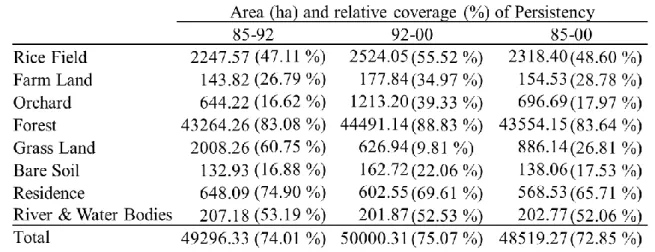
5.5.1 Persistency of Land Cover Maps………..59
5.5.2 Gains/Losses, Net Change and Net Change Contributions……..60
5.5.3 Net Change of Land Cover Maps……….62
5.5.5 Contributions to Net Change vs Elevation………...69
5.5.6 Contributions to Net Change vs Slope………..75
5.5.7 Cause of Changes………..…....81
Chapter 6.
Discussion……….……85
6.1
Preprocessing Stage………..…85
6.2
Evaluation of Land Cover Maps Production………....86
6.3
Change Analysis Assessment………..….93
Chapter 7.
Conclusion………...97
Acknowledgement………....103
List of Figures
Figure 1 Total population of farmer in Japan between 1985 and 2010 ... 5
Figure 2 Ratio of age of farmer in Japan between 1995 and 2010 (MAFF, 2012) .... 5
Figure 3 Total population of farmer in Hita City between 1985 and 2010 ... 6
Figure 4 Ratio of age of farmer in Hita City between 1995 and 2010 (MAFF, 2012) ... 6
Figure 5 Location of the study area (Hita City Oita Prefecture, Japan) ... 19
Figure 6 Analysis Flowchart ... 27
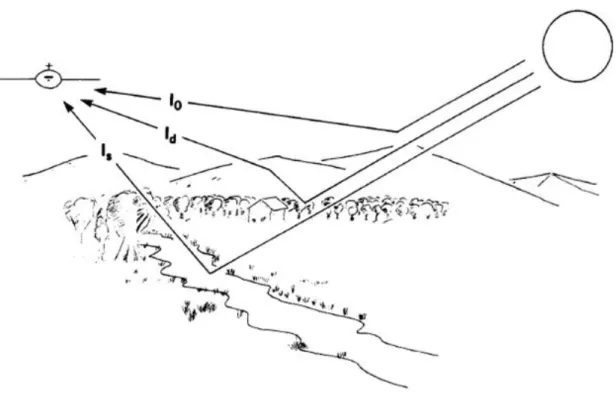
Figure 7 Schematic diagram of addictive components of atmospheric affects on remotely sensed data (based on Kaufman, 1984). Observed radiance at sensor (I) is sum of Is (radiance reflect from Earth’s surface), Io (radiance scattered from solar beam directly to sensor without reaching Earth’s surface), and Id (diffuse light- radiation reflected from Earth’s surface, then scattered to sensor) (Champbell and Ran, 1993). ... 31
Figure 8 Land cover map of 1985 ... 47
Figure 9 Land cover map of 1992 ... 48
Figure 10 Land cover map of 2000 ... 49
Figure 12 Net changes of all class between 1985 and 1992 ... 64
Figure 13 Net changes of all class between 1992 and 2000 ... 64
Figure 14 Net changes of all class between 1985 and 2000 ... 64
Figure 15 Net change contributions to Rice Field between 1985 and 1992 ... 66
Figure 16 Net change contributions to Farm Land between 1985 and 1992 ... 66
Figure 17 Net change contributions to Orchard between 1985 and 1992 ... 66
Figure 18 Net change contributions to Rice Field between 1992 and 2000 ... 67
Figure 19 Net change contributions to Farm Land between 1992 and 2000 ... 67
Figure 20 Net change contributions to Orchard between 1992 and 2000 ... 67
Figure 21 Net change contributions to Rice Field between 1985 and 2000 ... 68
Figure 22 Net change contributions to Farm Land between 1985 and 2000 ... 68
Figure 23 Net change contributions to Orchard between 1985 and 2000 ... 68
Figure 24 Net change contributions to Rice Field vs. elevations between 1985 and 1992 ... 70
Figure 25 Net change contributions to Farm Land vs. elevations between 1985 and 1992 ... 71
Figure 26 Net change contributions to Orchard vs. elevations between 1985 and 1992 ... 71
Figure 27 Net change contributions to Rice Field vs. elevations between 1992 and 2000 ... 72 Figure 28 Net change contributions to Farm Land vs. elevations between 1992 and 2000 ... 72 Figure 29 Net change contributions to Orchard vs. elevations between 1992 and 2000 ... 73 Figure 30 Net change contributions to Rice Field vs. elevations between 1985 and 2000 ... 73 Figure 31 Net change contributions to Farm Land vs. elevations between 1985 and 2000 ... 74 Figure 32 Net change contributions to Orchard vs. elevations between 1985 and 2000 ... 74 Figure 33 Net change contributions to Rice Field vs. slopes between 1985 and 1992
... 76 Figure 34 Net change contributions to Farm Land vs. slopes between 1985 and 1992 ... 77 Figure 35 Net change contributions to Orchard vs. slopes between 1985 and 199277 Figure 36 Net change contributions to Rice Field vs. slopes between 1992 and 2000
... 78 Figure 37 Net change contributions to Farm Land vs. slopes between 1992 and 2000 ... 78 Figure 38 Net change contributions to Orchard vs. slopes between 1992 and 200079 Figure 39 Net change contributions to Rice Field vs. slopes between 1985 and 2000
... 79 Figure 40 Net change contributions to Farm Land vs. slopes between 1985 and 2000 ... 80 Figure 41 Net change contributions to Orchard vs. slopes between 1985 and 200080 Figure 42 Rice Field changed into Grass Land occurred in remote areas from roads and rivers. ... 83 Figure 43 Gains and losses of Residence in Hita City between 1992 and 2000. Residence increased at a center of urban area and at places close to roads and rivers. ... 84
List of Tables
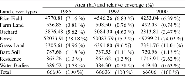
Table 1 Data Sets ... 20 Table 2 Classes of the mesh data and classes of this research ... 33 Table 3 Classes before the reclassification and classes after the reclassification .... 39 Table 4 Example of error matrix ... 42 Table 5 Area & relative coverage of land cover maps 1985 - 2000 ... 46 Table 6 Area & relative coverage of agricultural land classes v.s elevations in 1985
... 54 Table 7 Area & relative coverage of agricultural land classes v.s elevations in 1992
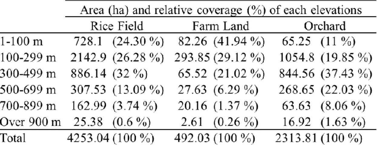
... 54 Table 8 Area & relative coverage of agricultural land classes v.s elevations in 2000
... 54 Table 9 Area & relative coverage of agricultural land classes v.s slopes in 1985 ... 57 Table 10 Area & relative coverage of agricultural land classes v.s slopes in 1992 . 57 Table 11 Area & relative coverage of agricultural land classes v.s slopes in 2000 . 57 Table 12 List of 56 types of change patterns related to agriculture ... 58 Table 13 Area & relative coverage of land cover maps persistency 1985 - 2000 ... 60 Table 14 Error matrix of land cover map in 1985 ... 90
Table 15 Error matrix of land cover change in 1992 ... 91 Table 16 Error matrix of land cover change in 2000 ... 92
Abstract
This research aims at examining the causes and features of the land cover change in Hita City using the spatial analysis decline, so as to understand its impacts on the agriculture in Hita.
Hita City is under a very severe situation: its population has decreased from 83,655 inhabitants to 71,555 between 1985 and 2010. The main reason for this is the decline in its basic industries, including forestry, agriculture and tourism. Focusing on the agricultural sector will be crucial to understand the inherent causes of decline in most of these industries in Hita City.
Main objectives of this research are therefore: (1) to map land cover changes in Hita City, especially in the agriculture and (2) to investigate on features and causes of dynamics in agricultural land cover change.
This research employs two Landsat TM data (2nd May, 1985 and 21st May, 1992) and one Landsat ETM+ data (17th April, 2000), vector data of administration boundary and vector data of lake in Japan for the geometric correction, vegetation maps as the ground truth and the digital elevation model. The analytical tool is the GIS software of IDRISI Taiga.
Analytical method in this research is for producing land cover maps consists of the following four steps: (1) Atmospheric correction of the satellite data, (2) Segmentation Classification, (3) Accuracy assessment and (4) Post-classification Comparison.
Overall accuracy of each land cover maps are 70.97%, 69.93% and 76.78%, respectively.
Net changes show all agricultural class decreased, forest decreased and glass land increased between 1985 and 2000. Net change contribution shows rice fields changed into glass lands and farm lands changed into residential areas between 1985 and 1992, rice fields and farm lands changed into residential areas between 1992 and 2000 and orchards changed into forests between 1985 and 2000.
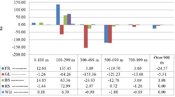
Net change contributions versus elevations shows land abandonments in rice fields mainly occurred in more than 300 m above from sea, land abandonments in orchards occurred in every elevation and urban development taken place to farm lands occurred in lower elevation between 1995 and 1992. Between 1992 and 2000, urban development taken place to rice fields and farm lands occurred in lower elevation and land abandonments in orchards occurred in a lower elevation than before. In the slope part, all of changes were distributed broadly, thus there was no features.
Roads and rivers show other features of land abandonments and urban developments. Land abandonment in rice fields between 1985 and 1992 occurred at remote areas from roads and rivers. Urban development occurred at places close to roads and rivers between 1992 and 2000.
This research shows the ecological divers which elevations and accessibility to roads and rivers contributed to land abandonments in rice fields. Hita City has been suffered by the depopulation issue and population aging issue both in total population and farmer’s population. There is a possibility that a market of Hita City shrank due to these issues and it caused land abandonments in agriculture.
In 1995, Hita City had a high way construction. There was a possibility that the construction caused the urban development and it made rice fields decrease in the city. On the other hands, Hita City has faced the depopulation issue, thus this urban development seems to be the development in infrastructure.
More detail and convince understanding of decline in agriculture is required. More additional change derivers are necessary to employ as future works. The integrated radio metric correction for the preprocessing and the filtering the classified image before post-classification comparison are also arose as future work to improve the accuracy of classification images and the change analysis.
Chapter 1. Introduction
1.1 Research Background
Agriculture in Japan has been declining due to land abandonment and urbanization, which in turn is essential for Japan’s food security and economic development. The Ministry of Agriculture, Forestry and Fisheries (MAFF) (2010) reported situations of agriculture and its villages in Japan are facing critical situations involving decreasing income of farmers, aging of famers, decreasing the total number of farmers, impoverished agricultural village, increase of abandoned agricultural landa and etc.
Agriculture performs multiple functions; stable food supply, maintaining soil and preventing soil erosion, watershed function, air purification, CO2 sequestration,
landscape for relaxing, conservation biodiversity and traditional value (Science Council of Japan 2001). Particularly, the traditional Japanese rural landscape in agricultural village owns Satoyama found between cities and deep mountains (Knight, 2010; Morimoto 2011). The landscape in Satoyama is, can be called as a heterogeneous landscape, a land-use mosaic. A different land use elements that generate this mosaic are interrelated to one another, and together form a cohesive system. The landscape has high value due to it providing a diversity of ecosystem services (Takeuchi, 2010).
However, in the last half-century, the role of rural landscapes in Japan has changed because of the shift from a rural-based to an urban-based in economic structure (Iwata et al., 2011). Tsurukawa and Ohno around Tokyo metropolitan areas had experienced urbanization since 1880 to 2001. Tsurukawa experienced rapid and drastic change into an urban landscape from a rural landscape, and in contrast, Ohno experienced a relatively gradual transition into former urban landscape from a rural land scape (Ichikawa et al., 2006).
On the other hand, land abandonment was widely observed in areas with difficult conditions for mechanized agriculture areas with difficult conditions for mechanized agriculture. It was caused by which modern impacts of an energy revolution and an introduction of chemical fertilizers, along with an economic growth which resulted in serious depopulation of the rural region, altered the structure of Satoyama landscape (Fukamachi et al., 2001). Traditional rural landscapes resulted in a great diversity of sustainable diversity. Rural landscape structure is essential for maintaining a biodiversity and a cultural diversity (Antrop, 2005).
In terms of food security, the agriculture plays a very important role. According to the MAFF, food self-sufficiency in Japan has gradually decreased from 73 % in 1965 to 39 % in 2011 on a calorie basis. Moreover the self-food sufficiency in Japan is much
lower than that of other countries, for example, among developed countries, USA’s was 130%, Canada’s was 223%, Germany’s was 93 %, Great Britain’s was 65 % and Italy’s was 59 % in 2009.That of Japan in 2009 was 40%. The MAFF in Japan set the goal of increasing their self-food sufficiency in the calorie basis for 45 % until 2015. Hence revitalization in the agriculture is required (MAFF, 2009).
This research investigates the agriculture in terms of agricultural land changes. Thus an investigation of agricultural land changes shows a mechanism of decline in the agriculture. Results of our research will contribute to understanding the agriculture in Japan.
1.2 Problem Statement
A decline trend is observed in agriculture of Japan derived from a statistical data. According to the census of the MAFF, the total number of population engaged in agriculture had decreased dramatically from 4,228,732 in 1985 to 2,527,948 in 2010 (Figure 1). The ageing of farmers is another problem in agriculture. A ratio of farmers over 60 years old was 29.01 % in 1985, however it increased 47.14 % in 2000 (Figure 2).
In Hita City, Oita Prefecture, more severe decline trend in its agriculture has been observed. The total number of population engaged in agriculture decreased from 31,907 to 9,009 between 1985 and 2000 (Figure 3). The ratio of farmers over 60 years old increased from 43.52 % to 73.43 % between 1985 and 2000 (Figure 4). Generally, Hita City is under a very severe situation: its population has decreased from 83,655 inhabitants to 71,555 between 1985 and 2010. A main reason for this issue is a decline in its basic industries, including forestry, agriculture and tourism (Hita City, 2011). Focusing on the agriculture will be crucial to understand the inherent causes of decline in most of these industries in Hita City. Understanding the decline of agriculture in Hita City contributes to understanding that in Japan.
Figure 1 Total population of farmer in Japan between 1985 and 2010
(MAFF, 2012)
Figure 2 Ratio of age of farmer in Japan between 1995 and 2010 (MAFF, 2012)
1985 1990 1995 2000 2005 2010 4,228,738 3,834,732 3,443,550 3,120,215 2,848,166 2,527,948 2,000,000 2,500,000 3,000,000 3,500,000 4,000,000 4,500,000 21.39 18.80 17.81 18.49 17.47 14.90 49.60 47.19 43.89 40.96 39.88 37.96 8.27 10.30 9.88 8.20 7.24 9.26 20.74 23.72 28.41 32.34 35.42 37.88 0% 10% 20% 30% 40% 50% 60% 70% 80% 90% 100% 1985 1990 1995 2000 2005 2010 Over 65 60~64 30~59 16~29
Figure 3 Total population of farmer in Hita City between 1985 and 2010
(MAFF, 2012)
Figure 4 Ratio of age of farmer in Hita City between 1995 and 2010 (MAFF, 2012)
1985 1990 1995 2000 2005 2010 31,907 29,378 25,115 22,869 11,083 9,009 5,000 10,000 15,000 20,000 25,000 30,000 35,000 10.10 7.36 6.27 7.56 5.14 3.90 46.38 39.75 32.53 26.87 25.74 22.66 14.01 17.58 14.38 11.18 10.37 11.54 29.51 35.31 46.82 54.39 58.76 61.89 0% 10% 20% 30% 40% 50% 60% 70% 80% 90% 100% 1985 1990 1995 2000 2005 2010 Over 65 60~64 30~59 16~29
1.3 Preliminary Research
Change of agricultural lands in Hita City between 1976 and 2006 was investigated based on Land Cover Map using GIS (Geographic Information System) technique. The data set consists of 5 periods of Land Cover Maps published by the Ministry of Land, Infrastructure, Transportation and Tourism (MLITT) in 1976, 1987, 1991, 1997 and 2006. The results of our preliminary research show that 913 ha of agricultural lands had changed into forests between 1997 and 2006.
However, there are two problems concerning the Land Cover Map derived by MLITT: low spatial resolution (100m) and only one vegetation category of forests. Agricultural land in Japan normally has an area of less than 100×100 m2. Therefore, the spatial resolution is not enough to distinguish agricultural lands accurately. This implies the need of higher resolution (less than 100 m) data in order to conduct this research. Moreover, it is very clear that just one category for vegetation covers is not sufficient for a detailed research on land cover changes.
1.4 Problems in the Preliminary Research 1.4.1 Spatial limitation
A spatial resolution of the mesh data is 100m ×100m. According to a traditional measurement of agricultural land in Japan, 1 Tan is its usual measurement, which equivalent 991.735537 m2. Agricultural land area in Japan is consisted by around 10 a. Thus the spatial resolution of the mesh data is need to enhance to investigate the agriculture in Japan.
1.4.2 Category limitation
The mesh data produced by MLITT is consisted by 10 categories land cover: Rice Field, Farm Land, Forest, Waste Land, Urban Area, Transportation & Network, Other Built Area, River & Water Bodies, Beaches and Sea. The mesh data works well to investigate a rough dynamics of land cover changes or the coastal area on the ground of categories of Beach and Sea does not work in an inland area. Moreover, the “Forest” vegetation category is inadequate for this purpose. More detailed categorization is required. The agriculture involves varieties of vegetation, for example, grass land, deciduous forest, coniferous forest, evergreen forest and etc. For more deeply
understanding of the agriculture, the more detailed vegetation categories are essential. Hence the more detailed vegetation categories contributes to obtain the great understanding of the dynamics of land cover change in agriculture.
1.5 Research Objective
Main objectives of this research are: (1) to map land cover changes in Hita City, especially in the agriculture and (2) to investigate on features and causes of dynamics in agricultural land cover change.
The investigation from more precise and specific land cover maps will contributes to the effective policy making of agriculture in Hita City and Oita prefecture and the revitalization of its agro-industry.
Chapter 2. Literature Review
2.1 Change Detection
Singh (1988) defines change detection is the process of identifying difference in the state of an object or phenomenon by observing it at different temporal scale.
Lu et al. (2004) states timely and accurate change detection of Earth’s surface features provides the foundation for better understanding relationships and interactions between human and natural phenomena to better manage and use resources. The monitoring of change Earth’s surface features is becoming important so that change detection research technique is an active topic and new developed techniques are arisen constantly.
Coppin et al. (2004) states, in the change detection, removing noises is essential process because inherent noises produce unreal change phenomena and inaccurate outcomes. Unreal change phenomena is caused, among two different satellite, by difference in atmospheric absorption and scattering due to variations in water vapor and aerosol concentrations of the atmosphere at temporal difference, temporal variations of solar zenith and azimuth angle, and inconsistent sensor calibration at time difference. Coppin et al. (2004) also states methodology of change detection has been developed for long times. There are various techniques and these are categorized as Algebra, Transformation, Classification, Advanced Model and etc. Algebra includes the image
differencing, the image rationing, the vegetation index differencing, the change vector analysis and the background subtraction. Transformation includes Principal component analysis, Kauth-Thomas transformation, Gramm-Schmidt and Chi-square transformation. Classification includes Post-classification comparison, Spectral-temporal combined analysis, Expectation maximization algorithm change detection, Unsupervised classification comparison and Hybrid change detection. The advanced models include Li-Strahler reflectance models, Spectral mixture models and Biophysical models.
Lu et al. (2004) recommends selecting the suitable change detection technique for obtaining the achievement of the research. For example, the visual interpretation of multi-temporal image color composite is a valuable technique for rapid qualitative change detection, the single band differencing and the principal component analysis are good method for obtaining change/non-change information and the classification is recommended technique for analyzing a detail from-to change detection if sufficient ground truth data are available.
2.2 Atmospheric Correction
Song et al. (2001) compared several atmospheric correction methods; Dark Object Subtraction, Dense Dark Vegetation, Modified Dense Dark Vegetation, Path Radiance and Relative Atmospheric Correction. According to results of this research, simple atmospheric correction algorithms such as Dark Objective Subtraction or Relative Atmospheric Correction is recommended for change detection and analyzing large numbers of images.
2.3 Land Cover Change as related to Agriculture
Peterson and Aunap (1998) found that the one third of the agricultural lands in Estonia had been abandoned between 1990 and 1993 using the multi seasonal Landsat Multispectral Scanner sensor (MSS) data. They successfully discriminated the agricultural land and other land use by the thresholding and the discrimination in in their classification process and they also employed the principal component analysis to enhance the differentiation with the ploughed land, the grass land and winter crops. However they failed to discriminate the grass land and the successional old field.
Kepner et al. (2000) investigated the land cover change in southeast Arizona, northeast Sonora and Mexico between 1973 and 1992. They found that a grass land and a desert scrub are the most vulnerable ecosystems and invaded by a xerophytes’ mesquite woodland. The number of grass land and desert scrub patches increased, however these patches size decreased. In the contrast both the size and number of xerophytes’ mesquite woodland patches increased. They employ the unsupervised classification technique and produced maps with 60 spectrally distinct classes, and then 60 classes were reclassified for 9 classes based on the ground truth reference and their field survey.
Kuemmerle et al. (2006) produced the land cover maps from the Landsat Thematic Mapper (TM) and the Landsat Enhanced Thematic Mapper Plus (ETM+) in the Polish, the Slovak and the Ukrainian Carpathian Mountain using a hybrid classification technique for the classification and compared land covers of these tree countries. Overall accuracy of their production was 84 %. They obtained the results which the Poland had about 20 % more forest cover at higher elevation than the Ukraine. Ukraine had the high agricultural fragmentation and the widely spread early successional shrub land derived by the land abandonment. They also found these results suggest that broad-scale socio economic and politics are the major significance factor for the land cover change in Eastern Europe.
Pôcas et al. (2011) found that meadow areas in increased 60 % and annual crops decreased 43 % between 1979 and 2002 in the Northeast Portugal. Reasons of increase of meadow are the policy supporting to the agro-environmental conservation and livestock production. On the other hand, reasons of decreasing annual crops are a loss of economic competitiveness in main annual crops, a population decrease and an aging issue in rural area, these induced the land abandonment. They used the satellite data of the Landsat MSS for 1979, the Landsat TM for 1989 and the Landsat ETM+ for 2002. They employed the supervised classification technique in the classification stage and radiometric information and Normalized Difference Vegetation Index (NDVI) in the training stage. Their land cover maps had 11 classes and marked high overall accuracy above 92.5 %.
2.4 Change Analysis
Kuemmerle et al. (2006) investigated land covers in the Polish, the Slovak and the Ukrainian Carpathian Mountain using Landsat TM and Landsat ETM+ data and compared with three countries’ land covers distribution and its elevation levels in the analysis part. This research also employs the fragmentation component in tree classes;
Forest, Arable Land Grass Land. This research found the broad-scale socio economic and politics are the major significance factor for the land cover change in Eastern Europe.
Forkuor and Cofie (2011) investigated land cover changes among Agricultural land, Low Built-up, Grass Land, Evergreen Forest and Barren Land and observed urbanization, land abandonment and deforestation. A linkage of between these types of phenomenon was proved by a key information interviews and observations in field visits.
Weng (2002) investigated land cover changes in the Zhujiang Delta using 7 land cover classes; Urban or Built-Up, Barren Land, Crop Land, Horticulture Farms, Dike-pond Land, Forest and Water. This research found that a rapid urbanization and crop lands loss occurred in that area. This research also employed additionally calculating transition probabilities of land covers.
Onur et al. (2009) investigated that land cover changes in Kemer, Turkey using 5 land cover classes; Urban fabric, Heterogeneous agricultural lands, Permanent crops, Forests, Open spaces with little or no vegetation, and Inland waters. This research observed that urban settlements increased by 159 % between 1985 and 1997 due to population increase and population increase were caused by tourism.
Mallinis et al. (2011) mapped and interpreted historical land cover land use changes in Nestos delta, Greece between 1945 and 2002 using 8 land cover classes; Agricultural lands, Barren lands, Urban or built-up areas, Forest lands, Range lands, Inland waters, Wet lands and Sea. This research also investigated gross gain, gross loss, persistence, swap, net change and total change in each class. As the results of research, a decline trend in agricultural lands was observed while afforestation and natural establishment occurred. It assumed to be caused by a policy change or agricultural population aging.
Díaza et al. (2011) investigated a relationships between land abandonments and indicators; Soil, Farm subsidy, Distance to second road, Distance to municipality’s capital, Distance to national park, Distance to aquaculture centers, Amount of bovine heads, Carrying capacity of farm pastures, Amount of Forest cover, Farmer’s age, Farmer’s education level and Residency status of land owner. This research showed soil quality was a significant benefit related geophysical driver of land abandonment. Important drivers in socioeconomic drivers were the distances to secondary roads, aquaculture production centers, and national parks, and the existence of farm subsidies. Significant farm structural variables were the amount of bovine heads and farm’s livestock carrying capacity. Status derivers such as age, education, and place of residence of the farmer were not significant.
Reis (2008) interpreted land cover changes in Rize, northeast Turkey between 1976 and 2000 using 7 claases; Bare soil, Agriculture, Deciduous, Coniferous, Pasture, Urban and Water. This research also employed elevations and slopes to investigate land cover changes features. This research found an increase trend in agriculture and a decline trend in forest. In the low slope regions, these changes were observed.
Hepcan et al. (2011) monitored land cover changes in the Cesme coastal zone, Turkey using 5 classes; Natural land cover, Agriculture, Built-up, Lake and Beach. This research found that urbanization occurred while natural land cover and agriculture decreased. The urbanization was caused by development of high way transportation.
Chapter 3. Research Design
3.1 Study area
Hita City is located in the western part of Oita prefecture, between latitudes 33˚27 and 33˚01 and longitudes 130˚49 and 131˚05 (Figure 5). The city is surrounded by the Mt. Aso, Kuju mountain range and Mt. Hiko. The Hita City has 19 mountains which all mountains are higher than 800 m and the 8 out of 19 are higher than 1000 m. These mountains produce the rich water resource and it meets in the Hita basin then supplied for the Fukuoka city. The range of the elevation in Hita City is between 1231 m and 38 m from sea level. The highest temperature was 38.6 degree in Celsius and the lowest temperature was -6.2 degree in Celsius in 2006. Its annual average temperature was 15.8 degree in Celsius in 2006. The annual precipitation was 1984 mm in 2006 (Hita, ).
Hita City integrated Hita county Oyama town, Amagase town, Maetsue village, Nakatsue village and Kamitsue village in 2005. The definition of Hita City in this research is after 2005.
Figure 5 Location of the study area (Hita City Oita Prefecture, Japan)
3.2 Data Sets
Data sets are consisted by three satellite data, four vector data, three vegetation maps and the digital elevation model and the IDRISI Taiga which is the GIS software is used for the analytical tool (Table 1). The satellite data which are 1985, 1992 and 2000 are adjusted to vegetation maps of 1983-1985, 1990-1995 and 2000-2007, respectively.
Table 1 Data Sets
3.2.1 Satellite Data
Satellite data is provided by a satellite system launched for an earth surface observation. There are several satellite systems; The Satellite Pour l'Observation de la Terre (SPOT) is provided by the French government and its first satellite was launched
in February 1986 (SPOT, 2012), the Moderate Resolution Imaging Spectroradiometer (MODIS) carried on the Terra Satellite (launched December 18th, 1999) and Aqua Satellite (launched May 4th, 2000) is provided by the National Aeronautics and Space Administration (NASA) (NASA, 2012), AVNIR-2 carried on the Advanced Land Observing Satellite (ALOS) are provided by theJapan Aerospace Exploration Agency (JAXA) and it was launched in January 24th, 2006 (JAXA, 2012), the Landsat was provided by NASA and its first satellite was launched in July 23rd, 1972 (USGS, 2012). This research uses two Landsat TM’s data (May 2nd 1985, May 21st 1992) and a Landsat ETM’s data (April 17th 2000). Two Landsat TM data are row data. A processing level of Landsat ETM+ is L1T level. It is an overall geometric fidelity of the standard level-one terrain-corrected product using ground control points and a digital elevation model. These Landsat data own the same spatial resolution (30 m × 30 m) and seasonal similarity. For better spatial resolution in land cover map than the mesh data derived by the MLITT (100 m ×100 m), selecting Landsat data has an advantage, because Japanese traditional measurement in agriculture land is explained as Tan which is about 991.7 square meters. For better discrimination of land cover types at vegetation and agriculture than the mesh data, Landsat achievement also has advantage in terms of its owing multi-spectral bands. This research uses Landsat 6 bands which are from band
1 to band 5 and band 7 in a classification stage.
In order to investigate long term land cover change in the study area over several years, Landsat achievement is suitable and convince. Landsat TM achievement had been available since 16th July, 1982 until 15th June, 2001 and Landsat ETM+ achievement had been available since 15th April, 1999 and now on. However, image acquisition via the ETM+ was greatly impacted by system failure in scan line corrector in 31st May, 2003 (Lillesand et al., 2007). From above, Landsat achievements cover more than 20 years term. Thus Landsat data has an advantage at long term investigation.
From these reasons, using Landsat data is suitable for this research.
3.2.2 Vegetation Maps
Vegetation maps have been provided by the Ministry of Environment (MA) and created based on the vegetation survey of the MA for more than 30 years. The purpose of the survey is to understand the distribution and exist of vegetation in terms of a scientific view. First vegetation survey was taken place by field survey and the analysis of aerial photograph in 1973 and the 1/200,000 scale model of vegetation map was created. The MA produced the more detail vegetation map (1/50,000 scale model) based on second survey (1979) and third surveys (1983-1986) had been produced. Fourth
survey (1989-1993) and fifth survey (1994-1998) had been taken place based on a satellite data analysis and procedures of these surveys were to revise latest vegetation map based on the survey. In the fourth and fifth survey, Landsat products were used for it (MA, 1994). Since 1999 until 2003, sixth vegetation survey was taken place by the field survey and the analysis of satellite data. The sixth survey produced the more detail vegetation map than before. It was 1/25000 scale model. Until 2002, Tokyo Datum had been used as Japanese geodetic system. However, Survey Act in Japan was revised and a World Geodetic System (WGS) was introduced, in 2002, since then it has been facilitated to use as an alternative geodetic system in Japan (Goto, 2007). Vegetation data created before 2002 is adapted to the WGS (MA, 2012).
In this research, vegetation maps created in the third, fourth and sixth vegetation survey were used for the ground truth (MA, 2012).
3.2.3 Digital Elevation Model
Digital Elevation Model (DEM) is a topographical data and sometimes explained as the Digital Terrain Model (DTM). The DEM is a digital image. DEM owns the Digital Number (DN) value at pixels representing a surface elevation instead of a radiance
value from the earth surface. The DEM owns a surface elevation at pixels rather than radiance value (Lillesand, 2007).
This research employs the DEM derived from the ASTER Global Digital Elevation Model (GDEM). ASTER GDEM is provided by the Ministry of Economy, Trade, and Industry (METI) of Japan and the United States National Aeronautics and Space Administration (NASA). Data is collected from the Advanced Spaceborne Thermal Emission and Reflection Radiometer (ASTER), a space borne earth observing optical instrument. The spatial resolution of ASTER GDEM is 30 m × 30 m (ASTER GDEM, 2012).
3.3 Analytical Tools
All of analytical steps in this research are analyzed by the IDRISI Taiga which is provided by Clark Laboratory in the Clark University, United State America. IDRISI is the strong at the raster image analysis and satisfy the needs of GIS and remote sensing; data base query, spatial modeling, image enhancement, land change modeling and time series analysis, multi-criteria and multi-objective decision support, risk analysis, simulation modeling, surface interpolation and statistical characterization. It contains
more than nearly 300 program modules which make the input and output, the display and the analysis of geographic data possible. The IDRISI Taiga is comprehensive program and strong program to treat the spatial data (Clark Labs, 2012; Eastman, 2009).
Chapter 4. Methodology
4.1 Methodology Flow
Methodology shows satellite remote sensing, geometric correction & atmospheric correction, land cover map, accuracy assessment and change analysis. In the land cover map part, the segmentation classification and the maximum likelihood are used. A classification error matrix is employed as the accuracy assessment. This research uses two Landsat data TM data, a Landsat ETM data, three vegetation maps and four vector maps. IDRISI Taiga is used as the analytical tool. An overall methodology in this research is explained in the flowchart (Figure 6). All remote sensing products employ the Universal Transverse Mercator Geographic Coordinate System as reference system.
Figure 6 Analysis Flowchart
4.2 Satellite Remote Sensing
Lillesand et al. (2007) mention that Remote Sensing is the science and art of obtaining information about an object, area or phenomenon through the analysis of data acquired by a device that is not in contact with the object, area, or phenomenon under investigation. Eastman (2009) explains the remote sensing stunning that our eyes are excellent example of a remote sensing device. It is possible to gather information about
our surrounding by gauging the amount and nature of the reflectance of visible light energy from some eternal source (such as the sun or a light bulb) as it reflects off objects in our field of view. Satellite remote sensing is the remote sensing form space. It has made a possibility to observe the earth surface without the direct investigation such as a field observation. Hence, this technique allows investigating environment issues around the world while saving research cost and time.
However some difficulties are behind the satellite remote sensing technique. For example, the geometrical distortion exists in acquisition of raw satellite data, the atmosphere influence to electromagnetic waves which are captured in a remote sensing satellite sensor. Thus, solving these problems is necessary to acquire accurate results from using the remote sensing technique.
4.3 Geometric Correction
In the raw image, the geometrical distortion is contained. Hence it is essential that the accuracy geometric information registers to the satellite data. This procedure is the geometric correction.
There are two types of geometric corrections process. These basically depend on the type of distortion, systematic or random. The systematic distortion is easily corrected by using formula derived by the calculation from the mechanism and source of distortion. The random distortion is corrected by analyzing Ground Truth Points (GCTs) and picking these points up from the image. GCTs should be on the distinct shorelines or edge lines.
The two Landsat TM data does not contain the geometric information. Therefore the geometric information needed to be registered in two Landsat TM data as same information as the Landsat ETM+ data. The process of geometric registration uses linear equation for the establishment of a rubber sheet transformation, as if one of the grids were placed on rubber and warped to make it correspond to the other. The actual process is one in which a new grid is constructed and a set of polynomial equations is developed to describe the spatial mapping of data from the old (input) grid into the new (output) one. The input grid is then filled with data values by resampling the input grid and estimating, if necessary, the output value. In this case, the input grid is two Landsat TM data and the output grid is the Landsat ETM+ data. An interpolation method in the resampling process employs a nearest neighbor.
4.4 Atmospheric Correction
Atmosphere affects the satellite data. Lillesand (2007) states as at the molecular level, atmospheric gases causes Rayleigh scattering that progressively affect shorter wavelengths. He also states the major atmospheric components causes absorption of energy at selected wavelength. Thus the atmospheric correction is required to reduce the effect of atmospheric to the wavelength for obtaining the accurate satellite data.
This research employs the dark object subtraction for the atmospheric correction. This procedure of atmospheric correction is the simplest technique. According to the Champbell and Ran (1993), the technique is premised on that it is possible to approximate Io (radiance scattered from solar beam directly to sensor without reaching Earth’s surface) by locating dark object enough that Is (radiance reflect from Earth’s surface) is at nearly 0, so that the observed brightness in dark object estimates Io. Estimated Io in all band are subtracted from all values in the image. Then it is assumed that all values are close to the value without Io (Figure 7). Thus the effect from the atmospheric is removed from the image by this procedure.
Figure 7 Schematic diagram of addictive components of atmospheric affects on
remotely sensed data (based on Kaufman, 1984). Observed radiance at sensor (I) is sum of Is (radiance reflect from Earth’s surface), Io (radiance scattered from solar beam directly to sensor without reaching Earth’s surface), and Id (diffuse light- radiation reflected from Earth’s surface, then scattered to sensor) (From
4.5 Land Cover Map
Producing land cover maps is essential step to achieve the goal of this research. This research used the classification methodology to investigate that the agricultural land changes into what. In Chapter 1, the category of mesh data derived by MLITT is needed to enhance, particularly the vegetation part. Thus our land cover maps production involve additional vegetation category.
Data of this research are Landsat TM and ETM+ satellite data for the classification. In the classification stage, bands 1 to 7 (except 6) were used for processing.
Segmentation Classification approach for taking the training sites and Maximum Likelihood approach for the classification were conducted to produce the land cover maps.
4.5.1 Land Cover Classes
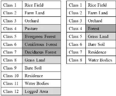
Before the classification, deciding land cover classes used in the research is required. The mesh data derived by MLITT is consisted by 10 classes; Rice Field, Farm Land, Forest, Waste Land, Urban Area, Transportation & Network, Other Built Area, River & Water Bodies, Beaches and Sea Area (MLITT, 2011). Land cover classes in this
research are on the mesh data and added some vegetation category from vegetation maps. The mesh data has only one class in the vegetation. This research improves the classes of the mesh data in the vegetation sector and the agriculture sector. Classes used in this research are Rice Field, Farm Land Orchard, Pasture, Evergreen Forest, Coniferous Forest, Deciduous Forest, Grass Land, Bare Soil, Residence, River & Water Bodies and Logged Area (Table 2). Farm Land includes any agricultural lands except for the rice field and the orchard.
4.5.2 Segmentation Classification
Segmentation classification is conducted similar process as a hybrid classification. Three basic steps are involved in segmentation classification procedure. In a segmentation stage (1), pixels are grouped based on its homogeneous spectral similarity. Next, in the training stage (2), identifying training areas and numerical description of the spectral attributes of each land cover type of interest in the scene based on the segment. After taking training sites, in a classification stage (3), a segment based classification is a majority classifier based on the majority class within the segment. Eastman (2009) mentioned as Segmentation classification improves the accuracy of the pixel-based classification and produces a smoother map-like classification result while preserving the boundaries between segments.
However the classification process is done by the maximum likelihood classification in this research and band 1 to band 5 and band 7 are used for all process of this classification. Band 6 involves thermal information of the earth surface. Hita City has Hita Onsen and Amagase Onsen. These onsens have possibility to impact the surface temperature. Thus this research does not employ the band 6.
4.5.2.1 Segmentation Algorithm
Eastman (2009) states a segmentation algorithm as there are three steps involved in a watershed based image segmentation process: 1) derive a surface image; 2) delineate watersheds from the surface image; and 3) merge adjacent watersheds that meet stated standards to form image segments.
In the first step, derive surface image, a variance image is obtained from each bands of image layer. A window moves with a width and height and is specified by the user. Then it is centered at every pixel. The variance within the window is estimated and assigned to that pixel. The latest surface image for watershed delineation is a weighted average of all variance images from all band’s image layers, and the weight for each bands of layer is provided by the user. The window sizes can be chosen, however a 3 x 3 window often provides optimal results. Thus I use a 3 x 3 window.
In the second step, delineate watersheds, pixels within a homogeneous region let have small values (close to zero) while pixels located at the boundaries of homogeneous regions should be higher values. Those values are treated as elevation values of a digital elevation model. In this process, pixels are grouped into one watershed if they are within one catchment. Each watershed is assigned with a unique integral value as its identification number.
In the last step, merge watersheds, adjacent image segments may be merged to form a new image segment according to their spectral similarity. The iterative merging process takes place. Every image segment is looked up to identify its most similar neighbors with each iteration. In this process, image segments which together with its most similar neighbor form a pair of image segments as candidates for merging. If those pairs meet two criteria, these are merged. Two criteria are following. The first criteria is what segments must be adjacent and have similarity to each other. For example, image segment A is adjacent to three neighboring segments B, C, and D. Segment B is identified as the most similar neighbor with A. Image segment B is adjacent four neighboring segments A, D, E and F. If segment A is identified as the most similar neighbor with B, two image segments A and B become a candidate pair. The second criterion is what the difference of the two image segments in a candidate pair must be less than a threshold. All candidates are looked up and the ones that have a calculated difference less than a threshold are merged.
The threshold of marginalization is examined based on the similarity tolerance. The similarity tolerance takes the number between 0 and 100. A larger number, for example 100, provides very large segments in size. In this research, the similarity tolerance is set on 0 to take the small area of training sites. Thus images are segmented based on the
delineate watershed stage. It means the marginalization is not taken place in this research.
4.5.2.2 Training Sites
Taking training sites is one of the most important steps in the classification because process quality of taking training sites determines a success of classification, hence a value of training site’s information produced from an overall classification effort (Lillesand, 2007). Objective of taking training sites is to collect a set of the statistical information which describes the spectral response pattern for each land cover types for the classification.
In this research, training sites are taken on the segment basis and ground truths are vegetation maps, field research and composite images. Particularly, field survey and composite images are mainly used as ground truth information. Vegetation maps are used as subsidiary information.
4.5.3 Maximum Likelihood
From above, the segmentation classification is similar to the hybrid classification. Thus it involves both unsupervised classification stage and supervised classification stage. In the supervised classification stage, various classification approaches exist. These approaches are a heart of the supervised classification. Through these approaches, data sets are evaluated in the computer using the appropriate decision rule to identify what category each pixel belongs to (Lillesand, 2007). Examples of these approaches are Minimum Distance to Means Classifier, Parallelepiped Classifier, Maximum Likelihood Classifier and Decision Tree Classifier. In this research, Maximum Likelihood Classifier was used for the classification. Easteman defined likelihood as it uses the means and variance/covariance data of signatures to estimate the posterior probability that a pixel belongs to each class.
4.6 Reclassification of Land Cover Map
In this stage, reclassifying land cover maps was conducted due to which some land covers with similar spectral reflectance were mixed or miss-classified. Particularly, the miss-classification or the mixed in other category was observed among Evergreen
Forest, Coniferous Forest and Deciduous Forest and among Pasture, Grass Land and Logged Area. These categories were reclassified as the Forest and the Grass Land (Table 3). Logged Area is originally defined as the grass in the vegetation map (ME, 2012). Thus it was reclassified into Grass Land.
Table 3 Classes before the reclassification and classes after the reclassification
4.7 Accuracy Assessment
Accuracy assessment is an essential process for evaluating and assessing accuracy or reliability of final productions in classification process. Vegetation maps derived by the ME are employed to use as the ground truth information and more than 10000 sample
points are produced by the statistical random sampling on vegetation maps to obtain the ground truth points.
4.7.1 Classification Error Matrix
Error Matrix is one of the most common means of expressing classification accuracy. It compares the reference data which is called the ground truth and the classification product on the categories by categories basis. The shape of matrices is square with the number of columns and rows same as the number of categories. Various classification errors of omission (exclusion) and commission (inclusion) are expressed by the error matrix. In the Table 4, pixels of the ground truth map classified into land cover map’s categories are explained along the major diagonal of the error matrix. For example, in the table 4, pixels of the ground truth corresponding to the Rice Field category in the land cover map is 317, that of Farm Land categories is 21, that of Orchard category is 44 and it keeps running from upper left to lower right.
Omission errors correspond to non-diagonal column elements, for example of the omission error, 3 pixels of Residence category which should be classified into the Bare Soil are excluded from that of category. On the other hand, commission errors
correspond to non-diagonal row elements, for example of the commission error, 3 pixels of Residence category and 11 pixels of Farm Land category are included in the Bare Soil category.
Overall accuracy can be calculated from the error matrix. The overall accuracy is calculated by which the total number of reference pixels divided by the total number of correctly classified pixels (the sum of the diagonal numbers). Other accuracies that can be calculated from the error matrix are a producer’s accuracy and a user’s accuracy. The producer’s accuracy results from which the number of the ground truth’s pixels used for each category (the column total of each category) divided by the total number of correctly classified pixels in each category (the diagonal number in each category). The user’s accuracy results from which the number of land cover map’s pixels used for each category (the row total of each category) divided by the total number of correctly classified pixels in each category (the diagonal number in each category).
Table 4 Example of error matrix
4.8 Change analysis
In this research, Land Change Modeler (LCM) produced by Clark Laboratory and the digital elevation model are employed for the change analysis. The LCM is consisted by five model types; Change Analysis is for analyzing past land cover change, Transition Potentials is for modeling a potential for land transitions, Change Prediction is for prediction cause of change into the future, Implications is for assessing implications for biodiversity and Planning is for evaluating planning interventions for maintaining ecological sustainability.
This research uses the Change Analysis for the change analysis step. The Change Analysis automatically estimates gains and losses, net change, persistency and specific
transition of land covers from land cover maps production. This analytical tool also produces these data in both geography map and graphical form (Clark Lab, 2012).
A digital elevation map, road vector map and river vector map are employed for investigating the cause of land cover change.
Chapter 5. Results
5.1 Land Cover Maps
Based on the analysis flowchart in figure 6 and referring to composite images, field observation and vegetation maps as the ground truth, land cover maps of Hita City between 1985 and 2000 were successfully classified and created. RSM errors in geometric correction are Root Means Square (RMS) errors in two resampled images are 0.933209 in 1985 and 0.887966 in 1992. According to visual check, there is geological consistency between Landsat ETM+ data and Vector and DEM data.
Land cover maps are consisted by following 8 classes; Rice Field (RF), Farm Land (FA), Orchard (OR), Forest (FR), Grass Land (GL), Bare Soil (BS), Residence (RS) and Water Bodies (WB).
In 1985, RS was located in the center of the city. FL was distributed around the residence area in center of the city. RF was distributed from center of the city to its edges and along the valleys (Figure 11). OR was also distributed along the valleys and most of that was in center of the northern middle of the city. FR was distributed in whole of the city and the GL was located into the forest as like a variegated leaf. BS was distributed along rivers. WB ran from the southern and eastern area of the city to its western area (Figure 8). 78.18 % of the city was covered by the forest. Agricultural
classes covered 13.79 % of the city. The relative coverage of residential area, bare soil and water bodies were 1.3 %, 1.18 % and 0.58%, respectively (Table 5).
In 1992, RS and FL were distributed as same as that of 1985. RF was also distributed as almost same as that of 1985, however RF was occurred in the southern part of the city. OR had almost same distribution as that of 1985, but its density was higher than 1985’s and the southern part and eastern part of OR were gone. FR was also distributed in whole of the city and the GL was spread into the forest than 1985. BS and WB had same distribution with its 1985. WB ran from the southern and eastern area of the city to its western area (Figure 9). The relative coverage of forest decreased from 78.18 % to 75.2 %. That of agricultural classes also decreased form 13.79 % to 12.22 %. Grass lands covered 9.6 % of the city; it increased 4.64 %. The relative coverage of residential area, bare soil and water bodies were 1.3 %, 1.11 % and 0.58%, respectively (Table 5).
In 2000, RS was spread in a concentric fashion in the center of the city and to valleys (Figure 11). FL was distributed as same as that of 1992. RF was also distributed as almost same as that of 1985, however RF took the place of by the residential area and bare soil. OR was gone around the residential area in the center of the city and remained near the rice field. FR was also distributed in whole of the city and the GL was more spread into the forest than 1992. BS spread around the residential in the center of the
city and in valleys. WB had same distribution with its 1992 (Figure 10). The relative coverage of forest decreased from 75.2 % to 74.02 %. That of agricultural classes also decreased form 12.22 % to 10.6 %. Grass lands covered 11.01 % of the city; it increased 1.41 %. The residential area increased two times than its in 1992. It increased from 1.3 % to 2.62 %. The relative coverage of water bodies was 0.63% (Table 5).
5.2 Accuracy Assessment of Land Cover Maps
Accuracy assessment employs the error matrix method in this research. The ground truth references are vegetation maps; Third Survey’s (1983-1986) for the land cover map in 1985, Fourth Survey’s (1989-1993) for the land cover map in 1992 and Sixth Survey’s (1999-2003) for the land cover map in 2000. Overall accuracy of land cover maps are 76.45 % in 1985, 74.54 % in 1992 and 77.73 % in 2000. Accuracy of these maps are higher than 74 %, thus these are acceptable (Congalton, 1991).
5.3 Land Cover Maps vs. Elevation
From now on, this research focuses on only agricultural classes. The relationship between the agricultural classes and elevations are explained.
In 1985, more than 60 % of RF and more than 90 % of FL was distributed blow the elevation between 1 m and 299 m. Both had the largest volume at between 100 m and 299 m, these were more than 50%. RF had the 31.92 % of its distribution at over 300 m. On the other hands, FL had only the 5.63 % of its distribution at the same elevation. OR had large volume between 100 m and 499 m, it was 85.49 % of its distribution. The largest volume of OR in elevation was between 100 m and 299 m (48.58 %). OR had
the 12.84 % of its distribution over 500 m. From these results, about 50 % of agricultural lands were distributed between 100 m and 299 m. At over 500 m, less than 15 % of agricultural lands were distributed. RF had the wider distribution at several elevations than other two types of agricultural lands (Table 9).
In 1992, more than 75 % of RF and more than 90 % of FL was distributed blow the elevation between 1 m to 299 m. Both had the largest volume between 100 m and 299 m, these were more than 57.85 % and 62.35 %, respectively. RF had the 22.94 % of its distribution over 300 m. On the other hands, FL had only the 8.66 % of its distribution at the same elevation. OR had large volume between 100 m and 499 m, it was 93.89 % of its distribution. The largest volume of OR in elevation was between 100 m and 299 m (60.34 %). OR had the 5.75 % of its distribution over 500 m. From these results, about 55 % of agricultural lands were distributed between 100 m and 299 m. At over 500 m, less than 7 % of agricultural lands were distributed. RF had the wider distribution at several elevations than other two types of agricultural lands (Table 10).
In 2000, more than 65 % of RF and FL was distributed blow the elevation between 1 m to 299 m. Both had the largest volume between 100 m and 299 m, these were more than 50.39 % and 59.72 %, respectively. RF had the 22.94 % of its distribution over 300 m. On the other hands, FL had the 23.57 % of its distribution at the same elevation. OR had
large volume between 100 m and 499 m, it was 83.09 % of its distribution. The largest volume of OR in elevation was between 100 m and 299 m (45.59 %). OR had the 14.64 % of its distribution over 500 m. From these results, about 50 % of agricultural lands were distributed between 100 m and 299 m. At over 500 m, less than 10 % of RF and FL and less than 15 % of OR were distributed. Agricultural lands had the same wide distribution at different elevations (Table 11).
Table 6 Area & relative coverage of agricultural land classes v.s elevations in 1985
Table 7 Area & relative coverage of agricultural land classes v.s elevations in 1992
5.4 Land Cover Maps vs. Slope
The relationship between the agricultural classes and slopes are explained.
In 1985, RF (94.96 %) was distributed less than 30º and 80.51 % of RF was distributed between 0º and 20º. The highest relative coverage of RF (32.14 %) marked between 10º and 20º. Over 30 º, only 5.03 % of RF existed. Most of FL (96.75 %) was distributed between 0º and 20º. The highest relative coverage of FL (55.04 %) marked between 0º and 5º. Over 30 º, only 0.4 % of FL existed. OR (98.47 %) was broadly distributed between 0º and 40º. Over 40º, only 1.53 % of OR existed. From these results, more than 80 % of RF and more than 95 % of FL were distributed between 0º and 20º. These two types of agricultural lands had the high density at that slope. OR was more broadly distributed at several slopes than other two agricultural lands. Over 50º, a little agricultural land exists (Table 12).
In 1992, RF (96.18 %) was distributed less than 30º and 84.12 % of RF was distributed between 0º and 20º. The highest relative coverage of RF (31.82 %) marked between 10º and 20º. Over 30 º, only 3.83 % of RF existed. Most of FL (96.28 %) was distributed between 0º and 20º. The highest relative coverage of FL (51.5 %) marked between 0º and 5º. Over 30 º, only 0.76 % of FL existed. OR (98.21 %) was broadly distributed between 0º and 40º. Over 40º, only 1.79 % of OR existed. From these results, more than
80 % of RF and FL were distributed between 0º and 20º. OR was more broadly distributed at several slopes than other two agricultural lands. Over 50º, a little agricultural land exist (Table 13).
In 2000, RF (95.67 %) was distributed less than 30º and 82.57 % of RF was distributed between 0º and 20º. The highest relative coverage of RF (32 %) marked between 10º and 20º. Over 30 º, only 4.34 % of RF existed. Most of FL (92.08 %) was distributed between 0º and 20º. The highest relative coverage of FL (41.94 %) marked between 0º and 5º. Over 30 º, only 1.63 % of FL existed. OR (98.37 %) was broadly distributed between 0º and 40º. Over 40º, only 1.64 % of OR existed. From these results, more than 80 % of RF and more than 90 % of FL were distributed between 0º and 20º. These two types of agricultural lands had the high density at gentle slope. OR was more broadly distributed at several slopes than other two agricultural lands. Over 50º, a little agricultural land exist (Table 14).
Table 9 Area & relative coverage of agricultural land classes v.s slopes in 1985
Table 10 Area & relative coverage of agricultural land classes v.s slopes in 1992
5.5 Land Cover Change Analysis
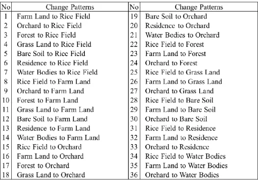
This research only focuses on changes of agricultural lands. According to land cover maps, decline trends of agricultural lands are observed between 1985 and 2000. RF, FL and OR decreased 224.55 ha, 28.35 ha and 792.18 ha between 1985 and 1992, respectively. Between 1992 and 200, RF, FL and OR decreased 293.22 ha, 16.47 haand 860.49 ha, respectively. The overall change of agricultural lands between 1985 and 2000 are what RF, FL and OR decreased 517.77 ha, 44.82 haand 1562.67 ha, respectively. I observed the 56 types of change patterns from the land cover change. The 36 changes out of 56 changes are related to the agriculture (Table 15).