E ffi cient Algorithms for Sign Detection in RNS Using Approximate Reciprocals

(1)

PAPER

Special Section on Cryptography and Information Security

E ffi cient Algorithms for Sign Detection in RNS Using Approximate Reciprocals

Shinichi KAWAMURA^{†,††,†††a)},Fellow, Yuichi KOMANO^††, Hideo SHIMIZU^††,Members, Saki OSUKA^††††,Nonmember, Daisuke FUJIMOTO^††††, Yuichi HAYASHI^{†††,††††},Members, andKentaro IMAFUKU^†††,Nonmember

SUMMARY The residue number system (RNS) is a method for representing an integerxas ann-tuple of its residues with respect to a given set of moduli. In RNS, addition, subtraction, and multiplication can be carried out by independent operations with respect to each modulus. Therefore, ann-fold speedup can be achieved by parallel processing. The main dis- advantage of RNS is that we cannot efficiently compare the magnitude of two integers or determine the sign of an integer. Two general methods of comparison are to transform a number in RNS to a mixed-radix system or to a radix representation using the Chinese remainder theorem (CRT). We used the CRT to derive an equation approximating a value ofxrelative to M, the product of moduli. Then, we propose two algorithms that efficiently evaluate the equation and output a sign bit. The expected number of steps of these algorithms is of ordern. The algorithms use a lookup table that is (n+3) times as large asM, which is reasonably small for most applications including cryptography.

key words: Chinese remainder, residue number system, sign detection, comparison

1. Introduction

RNS (residue number system) is a method for representing an integer xas an n-tuple of its residues with respect to a given set of bases {m1,m2,· · ·,mn}. The main fea- ture of RNS is that addition, subtraction, and multiplication can be carried out by independent addition, subtraction, and multiplication with respect to each base element, which en- ables fast computation via parallel processing. Due to this property, a lot of studies have been conducted to implement computation on integers with hundreds to thousands of bits, a size necessary for public-key cryptography, since around 2000[1],[2]. One reason for this timing is that an efficient base extension algorithm was proposed in[3], which is use- ful for implementing Montgomery multiplication in RNS.

However, how to efficiently compare magnitude of two integers or determine the sign of an integer in RNS is still an unsolved problem. Namely, comparison in RNS requires more computation steps than other operations such as multiplication. It is not unusual to avoid comparison in RNS.

Manuscript received March 16, 2020.

Manuscript revised June 12, 2020.

†The author is with ECSEC Technical Research Association, Tokyo, 101-0054 Japan.

††The authors are with Toshiba Corporation, Kawasaki-shi, 212-8582 Japan.

†††The authors are with National Institute of Advanced Industrial Science and Technology, Tokyo, 135-0064 Japan.

††††The authors are with Nara Institute of Science and Technol- ogy, Ikoma-shi, 630-0192 Japan.

a) E-mail: [email protected] DOI: 10.1587/transfun.2020CIP0020

For example, Bigou et al. studied the extended Euclidean algorithms, which require no comparison[4],[5].

General methods of comparison are classified into methods that either transform a number in RNS to a mixed- radix system (MRS) or to a radix representation using the Chinese remainder theorem. Garner proposed a method to transform RNS to MRS inO(n²) steps[6], which is regarded as the most efficient way among general methods. In fact, Knuth conjectured in his book that “there is little hope of finding a substantially better method [than Garner’s], since the range of a modular number depends essentially on all bits of all the residues” ([7], p.291. Words within [] were added by the present authors).

Vu proposed a sign-detection method that is more efficient than Garner’s in some restricted cases[8]. His idea is to evaluate x/M instead ofx, using the Chinese remainder theorem, where M = m1m2· · ·mn. Recently, a new sign- detection algorithm was proposed based on the Chinese remainder theorem[9], which is superior to any methods proposed before[9]. Both methods in[8] and[9] use lookup tables, which become enormous unless the bit size of the base elements is sufficiently small. Memory size for[9]is evaluated asO( log₂M3/(log₂log₂M)²) in bits.

We propose a new sign-detection algorithm based on the Chinese remainder theorem. In our algorithm, we evaluate 1/m_iby approximation and obtain a computational complexity ofO(n) with memory complexity,O

log₂M2 . We apply two approximation methods: one is based on a power series, and the other is based on a finite-length reciprocal table. In our algorithms, the approximation error is made smaller step-by-step until we can determine a sign bit. Once a sign is determined, the algorithm halts. Therefore, the number of computation steps can be limited. To make the algorithm implementation-friendly, we design it to be word- oriented.

A lot of research effort has considered specific sets of moduli such as{2^w+1,2^w,2^w−1}[10]–[13]. However, these moduli sets have relatively small size and do not necessarily fit to the optimization for fast cryptographic implementation such as[14]–[16]. Therefore, we focus on moduli sets that are scalable in size and easy to use for applications such as cryptography. The problem we try to solve is to propose a sign-detection algorithm that works for general bases with more efficiency and less memory than conventional algorithms.

Copyright c2021 The Institute of Electronics, Information and Communication Engineers

(2)

In Sect. 2, we describe the notation and background of our research. Section 3 explains the principle of our method.

We propose a method based on a power series in Section 4, and a method based on a reciprocal table in Sect. 5. Sec- tion 6 evaluates the computational complexity and memory size. Section 7 concludes the paper.

2. Notation and Background

2.1 Notation

The following notation is used in this paper.

w: the bit size of a word in a given computer.

hxim=xmodm, wherehxim∈[0,m).

BaseB={m₁, . . . ,m_n}, where gcd(m_i,m_j)=1(i, j).

Here, we assume mi=2^w−µ_i.

µ_iis an integer in the range, 0≤µ_i<2^bw/2c. M =

n

Y

i=1

mi

M_i=M/m_i Dx⁻¹E

mi

: a multiplicative inverse of x modulo mi, if gcd(mi,x)=1 holds.

{x}_B =hxi_m₁, . . . ,hxi_m_n: RNS representation ofx.

TransposeT: {x}^T_B =





 hxim₁

... hxim_n





 hxi_m⊗ hyi_m,hxyi_m

{x}_B⊗ {y}_B,{xy}_B=hxyi_m₁, . . . ,hxyi_m_n {x}B+{y}B,{x+y}B=hx+yim₁, . . . ,hx+yim_n A constantWassociated with baseB:

W=* ⁿ X

i=1

DM_i⁻²E

m_iMi

+

M

{W}_B = D M⁻¹₁ E

m₁, . . . ,D M_n⁻¹E

m_n

: The RNS representation ofW.

RNS(x): RNS representation ofx, not specifying a base.

MRS(x): MRS representation ofx, not specifying a base.

hxi₁ = x− bxc: A fractional part of a real number x. This is a natural extension of the symbolhxim =xmodm=x− mbx/mc, defined for integersx,m>1, since the right-hand sides coincide with each other ifm=1 is chosen.

x=bxc+hxi1

holds sincexis a sum of an integer partbxcand a fractional parthxi1.

For an arbitrary integera, the following equation holds:

haim

m =a m

1

.

Recall the relation below for proof.

a=m a

m +hai_m

The equation is apparent since ba/mcandhai_mrepresent a quotient and a residue ofa/m, respectively.

The dot product (or inner product) may be used for the algorithm description.

ha1 a2 . . . an

i





 x1

x2

... xn







=

n

X

i=1

aixi

k-bit right shift of an integerx:

xk=x 2^k

.

2.2 Sign Detection Based on MRS

We first define a sign function and a number with reverse sign.

Definition 1:

Let {x}_B be an RNS representation of an integer x ∈ [0,M−1]. A sign function of{x}Bis defined by

sign ({x}B)=











0, if x<M/2 1, if x≥M/2

Definition 2:

Let {a}_B be an RNS representation of an integera ∈ [0,M−1]. A number with the reverse sign of{a}Bis given by

{−a}_B ={M−a}B.

When Definition 1 is to be implemented, the problem is that the if-clause cannot be evaluated efficiently for a given{x}_B. Lety1, y2· · ·ynbe an MRS representation of a number represented as [x₁,x2· · ·xn] in RNS. Then the following equation holds:

x=y_nmn−1· · ·m1+· · ·+y₂m1+y₁.

In MRS, comparison of two integers can be carried out by comparing each digity_ifrom the most significant digit to the least significant one, as with ordinary radix representation. Therefore, we can compute a sign function as follows.

1. Convert RNS(x) to MRS(x) using Garner’s algorithm [4].

2. Compare MRS(x) with a precomputed value, MRS(dM/2e).

sign ({x}B)=











0, if MRS (x)<MRS(dM/2e) 1, if MRS (x)≥MRS(dM/2e)

(3)

The amount of computation necessary in each of the above steps is evaluated as the following.

Step 1. Modular multiplication:n(n−1)/2 times,

Step 2. Comparison ofw-bit words: Minimum once, maxi- mumntimes.

The most time-consuming part of this algorithm is modular multiplications, the number of which is estimated asO(n²). Note that in step 1, the first word computed is the least significant one, and the last word is the most significant one. Consequently, we cannot proceed to step 2 before computing all the words of MRS. As far as sticking to the basic operations permitted in RNS, there is no known comparison algorithm with complexity lower thanO(n²).

2.3 Sign Function andx/M

We can modify Definition 1 to derive Definition 3, in which equations in the if-clauses are divided by Mon both sides, without affecting the sign function.

Definition 3:

sign ({x}_B)=











0, if x/M <1/2 1, if x/M ≥1/2

According to Definition 3, we can efficiently compute the sign function ifx/M is evaluated efficiently from{x}_B. Let the binary representation ofx/Mbe defined by

x M =

∞

X

i=1

b−i·2⁻ⁱ,

whereb−i∈ {0,1}. Usually, the following relation holds.

b−1=0⇐⇒x/M<1/2 b−1=1⇐⇒x/M≥1/2

In this case, sign ({x}B) is given by the first bit after the decimal point ofx/M.

An exception can occur when x = M/2. If x/M is represented as 1·2⁻¹, then the rule above succeeds. But 1/2 can also be represented by a repeating decimal as

1 2 =

∞

X

i=2

1·2⁻ⁱ.

In such a case,b−1=0, and the above decision rule fails.

The Chinese remainder theorem is known as a way to compute a radix representation ofxfrom an RNS representation. The equation below is an expression of the Chinese remainder theorem

x=* ⁿ X

i=1

DxiM_i⁻¹E

m_iMi

+

M

, (1)

wherexi=hxim_i. If we divide both sides byM and replace a variable withξi=D

xiM⁻¹_i E

m_i, we obtain

x M =

* ⁿ X

i=1

ξ_i mi

+

1

. (2)

The right-hand side means an operation to provide the fractional part of the number in the parenthesis, or to truncate the integer part. By using{W}_B, defined in Sect. 2.1, we can expressξ_isimply as

hξ₁ ξ₂ . . . ξ_ni

={x}B⊗ {W}B.

We can construct a sign-detection algorithm by apply- ing (2) to the if-clause of Definition 3. This idea was first proposed in [8]. Although the equation evaluated in[8]is slightly different from (2) in that both sides are doubled (Equation (10) of [8]), its principle is the same as Theo- rem 1, which will appear in Sect. 3. In [8], the equation is evaluated using a lookup table, which has an entryξ_i/m_i with a precision of log₂nMbits, addressed byxi. Since the address isxi, the table entries become larger as the bit size of the base elements increases. Consequently, the application is limited to those with small moduli.

Recently, a new sign-detection algorithm with complexity O(n) was proposed in [9]. The algorithm uses a lookup table with very coarse precision. Nevertheless, it shares the same problem with the algorithm in[8], sincexi

is used as the address to a table entry. It is recommended in[9] that the base elements should be consecutive prime numbers starting from 3 to make the elements as small as possible.

For cryptographic applications, it is often the case that the bit length of each base element is chosen to be close to the word lengthwof a given computer to make each operation efficient. No sign-detection algorithm with a moderate table size has been proposed, even in such cases asw≥32.

Equation (2) is also used in[17], but procedure of sign detection is less efficient.

3. Principle of Proposal

3.1 Approximation Function

LetG(x) denote the value in the parenthesis of (2). Then, G(x)=

n

X

i=1

ξi

mi

.

In addition, the approximation ofGis denoted byG(x,d), where the second argument is a non-negative integer that represents the degree of approximation. We define the approximation error by

e(x,d)=G(x)−G(x,d).

We choose an approximation functionG(x,d) such that the following three conditions are satisfied.

(i) e(x,d)≥e(x,d+1)≥0 (ii) limd→∞e(x,d)=0 (iii) e(0,d)=0

(4)

This requires thate(x,d) decreases monotonically as d increases, thate(x,d)=0 withdinfinite, and that the error is 0 whenx=0.

Lete(d) be defined by e(d)=max

x e(x,d).

Then we obtain the following equation.

0≤e(x,d)≤e(d)

Conditions (i) and (ii) ensure that we can make the error as close to 0 as we like. Now we get Lemma 1 and Theorem 1.

Lemma 1:

If an approximation function and its error satisfy conditions (i) and (ii), there exists an integerδsuch that

0≤e(d)≤ε

holds for an arbitrary small real numberε >0 and all inte-

gersdsatisfyingd≥δ.

Theorem 1:

If the approximation errore(x,d) satisfies Conditions (i)–(iii), there exists an integerδsatisfying

e(δ)≤ 1 2M.

Then, for anyx∈[0,M−1] excludingx=M/2, the first bit after the decimal point of

hG(x, δ)i₁

is identical to that ofhG(x)i1, which equals the sign bit de-

fined in Definitions 1 and 3.

Refer to Appendix A for the proof. We exclude the casex= M/2 since there is a possibility that we cannot determine the sign byb−1 alone due to the occurrence of a repeating decimal. We will discuss how to deal with the casex=M/2 in Sect. 4.

3.2 Approximation Error and Sign Detection

We explain the mechanism to determine the sign of x fromhG(x,d)i₁. Figure 1 is a diagram showing the value of hG(x,d)i1 computed for a given x. Points P(x) = (x,hG(x,d)i₁) appear in the area between the lines y = (1/M)xandy =(1/M)x−e. In addition, they also appear in the triangular area above the liney =(1/M)x+(1−e).

Here, the symbol eis a simplified expression of the error bounde(d). To determine a sign, we first computehG(x,d)i1

from{x}_B, then evaluate the value according to the following rules:

hG(x,d)i1∈[0,1/2−e)⇒sign(x)=0, hG(x,d)i1∈[1/2,1−e)⇒sign(x)=1, hG(x,d)i1∈[1/2−e,1/2)∪[1−e,1)

⇒indeterminate.

Fig. 1 Diagram ofxversus approximatex/M.

IfhG(x,d)i1 ∈ [1/2−e,1/2) occurs from the indeterminate case, we can narrow the range ofxas ((1/2)−e)M ≤ x≤((1/2)+e)M. But, if P(x) is in the area C, the correct sign of xis 0. If, instead, P(x) is in the area A, the correct sign of xis 1. Thus, we cannot tell the correct sign. Simi- larly, ifhG(x,d)i1 ∈[1−e,1) occurs, we can only conclude that x ∈ [0,eM] or x ∈ [(1−e)M,M), and cannot determine the sign. We can rephrase the condition of Theorem 1, e(δ) ≤ 1/2M, as the condition that no point appears in the area A or in area C in Fig. 1. The analysis here also tells us that relatively high precision, or a largerd, is necessary for sign detection nearx = M/2, x=0, andx = M. Less precision, or smallerd, is required forxaway from them.

We will propose two candidates for the approximation functionG(x,d); one is based on a power series and the other is based on a reciprocal table.

4. Method Based on Power Series

To derive a concrete algorithm, the following three points should be considered.

• Choice of an approximation function that satisfies the condition in Theorem 1.

• Proposal of efficient algorithm to compute the approximation function.

• Moderate memory size.

4.1 Choice of Approximation Function

We pose a condition that is frequently used in the cryptographic implementation on the base elements, specifically,

mi=2^w−µi,

whereµ_i is an integer in the range 0 ≤ µ_i < 2^bw/2c andw is the bit size of a word for a given computer. With such a modulus, modular operations can be easily implemented.

(5)

Further optimization regardingµ_imay be possible for efficient implementation (e.g. [15]). The proposed algorithm can be combined with such optimization, if necessary.

The reciprocal ofmican be expanded as a power series 1

m_i = 1 2^w· 1

1−µ_i/2^w = 1 2^w

∞

X

k=0

µi

2^w k

.

Note that the equation holds for any case, includingµi=0, if we define 0⁰=1.

Substituting an infinite power series for the equation of G(x) and truncating the tail after thed-th power, we obtain the approximation function forG(x) as

G(x,d)=

n

X

i=1

ξ_i 2^w

d

X

k=0

µ_i 2^w

k

. (3)

The approximation errore(x,d) is given by e(x,d)=

n

X

i=1

ξ_i mi

µ_i 2^w

d+1

.

Ifxvaries,ξ_imoves in the range 0≤ξ_i≤m_i−1. Therefore, e(x,d) ranges in

0≤e(x,d)≤e(d)=

n

X

i=1

1− 1 m_i

!µi

2^w d+1

. (4)

Asd increases, the upper bound decreases exponentially.

This approximation fulfills the conditions (i)–(iii) in Sect. 3.

To simplify the expression ofG(x,d), we definegas g(x,k)=

n

X

i=1

ξi·µ^k_i. (5)

Then,G(x,d) is rewritten as G(x,d)=

d

X

k=0

1

2^w(k⁺¹⁾g(x,k). (6)

Next, we find a parameterd that is large enough for sign detection. Since M ≈ 2^nw, the following equation holds:

e(n−1)=

n

X

i=1

1− 1 mi

!µ_i 2^w

n

> 1 2^nw > 1

2M.

This means thatd=n−1 is not sufficiently large. Ifd=n, then

e(n)= 1 2⁽ⁿ⁺^1)w

n

X

i=1

1− 1 mi

! µⁿ_i⁺¹.

This implies there is a possibility thate(n) will satisfy the condition in Theorem 1 ifµiis small to some extent. In other words,d≥nis a necessary condition for the assumption of Theorem 1 to be fulfilled. Let us assume that we can findµi

andwthat satisfy the assumption of Theorem 1 ford =n.

Even if this is not true, we can make the error sufficiently small if we choose a bigger d. In this case, however, the number of computation steps increases as well. In addition, the termµ^k_i in (5) becomes larger and there is the possibility that an operation larger thanwbits is necessary.

Let us estimate the number of steps necessary to compute (3) ford = n. The number of terms that appear in a power series isnfor each base.nmultiplications are necessary to multiplynterms byξ_i. Since the suffixihasndiffer- ent values, we have O

n²

multiplications in total. This is not better than that of MRS. To improve the computational complexity, we must devise an efficient algorithm to evaluate the approximate equation.

4.2 SDPS Algorithm

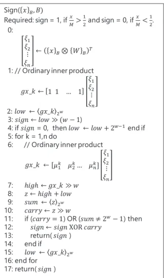
We propose a sign-detection algorithm based on Theorem 1 and name it SDPS (sign detection using a power series), the pseudocode of which is shown in Fig. 2. The variable gx kcorresponds to a function g(x,k) defined by (5). To computeG(x,d) efficiently, SDPS is designed according to the following policies.

• Computeµ^k_i in advance as a lookup table for 1/m_i.

• Start computing from the most significant word, which includes a sign bit.

• Stop computing as soon as a sign bit is determined.

These make it possible for the average number of computation steps to be O(n). To realize this, we must establish a way to decide whether the sign bit has been determined.

In Fig. 2, the algorithm stops either at step 13, in the middle of the for-loop, or at step 17, after the n-th loop is finished. At step 11, the if-clause is executed ifcarryequals 1 or sumis not all 1s. In the case when carry equals 1, carrytravels to the position of the sign bit,b−1, and the sign bit is fixed ever after. In the case when sumis not all 1s, sumwill not produce a new carry since a carry from the less significant block will stop withinsum. Hence, the sign bit is fixed in this case as well. The basis of this decision rule is the following simple property of carry propagation.

LetB,Cbe two binary numbers whosei-th bit is represented bybi,ci∈ {0,1}, respectively. The suffix is an integer and a larger suffix represents a more significant bit. Suppose biis the bit of interest andi> j. If a carrycjis added to the j-th bit of B, thenbichanges if and only ifcj =1 and all bits frombi−1tobjare 1.

The bit alignment of values computed in SDPS is presented in Fig. 3, where the left end is the decimal point and lower bits are located in the right-hand direction. In Fig. 3, low(0) andhigh(1) are added first, andsum(1) andcarry(1) are obtained. This procedure is continued to less significant blocks until the sign bit is fixed. In SDPS, the bit size of high(k) becomes bigger as the parameterkincreases due to the bit size ofµ^k_i. Ifhigh(k) becomes too big, SDPS will not give the correct sign. To circumvent such cases, we impose the following two conditions at step 7.

1. high(1)<2^w−1holds in the first loop

(6)

Fig. 2 RNS sign-detection algorithm SDPS.

2. high(k)<2^wholds in the later loops

Condition 1 ensures that the first bit ofhigh(1) after the decimal point is 0, which meanshigh(1) does not directly modify the sign bit. Condition 2 ensures that the carry at step 10 is at most 1. It is possible to prove that these conditions are satisfied if

e(n)≤ 1 2M holds (Appendix B).

Finally, we assert by Theorem 2 that the SDPS algorithm outputs the same result as computed byhG(x,n)i1. Theorem 2:

If e(n)=

n

X

i=1

1− 1 mi

!µi

2^w n+1

≤ 1 2M

holds, the return value of SDPS, except for the case x = M/2, is identical to the first bit after the decimal point of

hG(x,n)i1.

Fig. 3 Bit alignment of steps 1–10 of SDPS forn=3.

In addition, we can derive two corollaries that have simpler assumptions.

Corollary 1:

Theorem 2 holds even if we replace the assumption by

n

X

i=1

µⁿ_i⁺¹<2^(w−1).

Corollary 2:

Theorem 2 holds even if we replace the assumption by max (µi)ⁿ⁺¹·n<2^(w−1).

Proof is that from the assumptions of Corollaries 1 and 2, we can derive the following equation:

e(n)< 1 2^wn⁺¹ < 1

2M.

The assumption of Corollary 1 can be violated for large n unlessµ_iis adequately small. In Sect. 5, we will propose an algorithm with an easier constraint onµiso that the sign can be detected for a much wider range of bases.

4.3 Handling ofx=M/2

SDPS excludes the case thatx=M/2 for input. We consider how to deal with such a case.

1. Avoidx=M/2 by using oddM.

2. Use evenM, and return 1 if the input isx=M/2. We give three ways to determine the sign.

(a) Supposem1 is even. Then,x=M/2 can be represented as

{M/2}_B=[m₁/2,0, . . . ,0].

If this input is detected, return 1 immediately.

(b) Choosem₁ =2^w, that is,µ₁ =0, and run SDPS as usual. Then, SDPS returns 1.

(c) Choosem₁=2^w−µ₁, whereµ₁is a non-negative even number. In this case, SDPS computes 1/2 as a repeating decimal. We detect it by finding that the length of consecutive 1s is more thann words. This can be achieved by inserting the following code immediately

(7)

after step 14 of SDPS.

s1:ifk=nthen return(1) end if 5. Method Based on Reciprocal Table

5.1 Choice of Approximation Function

We propose an algorithm that has fewer restrictions on the parameterµithan SDPS. We assume that the base has a form explained in Sect. 2.1.

A reciprocal table is produced by dividing the reciprocal of a modulus represented in binary into a sequence of wordsh_i(k).

1 m_i =

∞

X

k=1

hi(k)·2^−kw 0≤hi(k)≤2^w−1

Substituting the table into (2) leads to x

M =* ⁿ X

i=1





 ξ_i

∞

X

k=1

hi(k)·2^−kw





 +

1

.

To distinguish a new approximation function fromG(x,n), we useH(x,d), which is defined as

H(x,d)=

d

X

k=1

h(x,k)·2^−kw

h(x,k)=

n

X

i=1

ξi·hi(k)

eH(x,d)=

∞

X

k=d+1

h(x,k)·2^−kw.

The upper bound of the error is estimated as eH(x,d)≤eH(d)<n·2^−(d−1)w.

This means that we can make the error as close to 0 as we like by taking sufficiently large d. Thus, we can find an integerδthat satisfies assumption of Theorem 1. If we take δ=n+2, it follows that

eH(n+2)<n·2⁻⁽ⁿ⁺^1)w.

In addition, ifnandwsatisfy the equation

n<2^w−1, (7)

we get

eH(n+2)<2^w−12⁻⁽ⁿ⁺^1)w=2^−nw−1< 1 2M.

This means that a sign bit is given by the first bit after the decimal point ofhH(x,n+2)i₁.

To efficiently evaluateH, we computehi(k) in advance.

The first two entries ofhi(k) can be written as

h_i(1)=1

h_i(2)=µ_i or µ_i+1

from analysis using a power series (Appendix C). We use these values to describe the algorithm in the next subsection.

The value ofhi(2) is described as ¯µi, which equalsµiorµi+ 1.

5.2 SDRT Algorithm

It takesO(n²) operations to compute a functionhH(x,n+2)i1

with full accuracy. To reduce the order, we propose an algorithm similar to SDPS that controls precision adaptively and halts as soon as the sign bit is fixed. We name this SDRT (sign detection using reciprocal tables). Pseudocode and the bit alignment of SDRT are shown in Figs. 4 and 5, respectively. As discussed in the previous subsection, it is necessary to take adequal to or larger than (n+2) so that the error is sufficiently small. In SDRT,dis set to (n+3) to simplify the description of the algorithm.

In SDPS, the boundary of words coincides with that of processing; that is, the variablesum(k) just fits between two word-boundaries in Fig. 3. In addition, it is a crucial point that the sign-detection at step 11 in Fig. 2 works correctly under the condition that thecarryis at most 1. On the other hand, if the boundaries of words and processing were made to coincide in SDRT, thencarrywould become at most 2.

In order to makecarryat most 1, we shift the boundary of processing by 1 bit to the decimal point. This makescarry at most 1 and the sign detection works correctly in Fig. 4.

To confirm thatcarryis at most 1, we first consider (7) and derive the following equation:

(h₃2w)<n<2^w−1. In addition, it is apparent that

hh1i₂w ≤2^w−1 hh2wi₂w≤2^w−1.

Then, we can estimate the maximum value oftmpat step 19 in Fig. 4 as less than 2^w+2^w−1+2^w−2−1. This proves that thecarryis at most 1. As a result, we can use the same code for steps 21–24 in Fig. 4 as used in steps 11–14 in Fig. 2.

LetS be the approximate value ofhH(x,∞)i1 derived from SDRT.S is computed by the summation of carries and sums that are aligned as shown in Fig. 5. SinceS is trun- cated at the{(n+1)w−1}-th bit after the decimal point, its approximation errore_RT is

eRT =hH(x,∞)i₁−S <2⁻⁽ⁿ⁺^1)w⁺¹< 1 2M.

SinceeRT satisfies the assumption of Theorem 1, we obtain the following Theorem.

Theorem 3:

Ifn <2^w−1, then for any integerx∈[0,M−1] except x = M/2, the return value of SDRT is identical to the first bit after the decimal point of

(8)

Fig. 4 RNS sign-detection algorithm SDRT.

hH(x,∞)i₁.

If x = M/2 occurs in SDRT, the same action as explained in Sect. 4.3 can be taken. As a special case, the action corresponding to 2-(c) is to insert the following code immediately after step 24 in Fig. 4.

s1:ifk=n+3then return(1) end if

Finally, we can solve the overflow-detection problem associated with addition efficiently by use of the sign func- tions proposed in Sects. 4 and 5 (See Appendix D).

Fig. 5 Bit alignment of steps 7-20 of SDPS forn=3.

6. Evaluation

6.1 Computational Complexity

6.1.1 Probability Derived fromd-th Approximation First, we derive the probability that a sign is determined from G(x,d). In this case, a residual error is bounded by e(d) from (4), while in SDPS, the error is bounded by a word boundary. Therefore, the probability derived here is not equal to that of SDPS, but the derivation process here will be applied to derive a probability of SDPS in the next Sect. 6.1.2. We assume that the distribution of input xis uniform.

From Fig. 1, the probability that sign ofxis determined is estimated as

ϕd=1−2e(d)

under the condition that the error ise(d).

Letp_ddenote the probability that a sign is determined when the d-th term is computed but not before this term.

Then, p_dis represented by p_d=ϕ_d−ϕ_d−1,

whered =0,1,2,· · · andϕ₋₁ =0. The upper bound of (4) leads to

p0=1−2

n

X

i=1

1− 1 mi

!µ_i 2^w

pd=2

n

X

i=1

1− 1 mi

!µ_i 2^w

d 1− µ_i

2^w

(d≥1).

p_d decreases exponentially as d increases. The expected number of operations can be computed using this probability.

6.1.2 Probability Derived from Error at Word Boundary Next, we derive probabilities representing SDPS and SDRT.

To represent both probabilities with a single formula, let us

(9)

Table 1 Number of operations in SDPS (left) and SDRT (right).

replace the loop variable with j. Let pjdenote the probability that a sign is detected at the j-th loop, where j = 0 corresponds to the process before the loop. For SDPS, jis the same as the loop variablekused in Fig. 2, whereas for SDRT, jandkhave the relationship j=k−2, from Fig. 4.

In SDRT, the maximum value of jis n+1, which is one larger than that of SDPS. In our analysis, we assume that pn+1 = 0. As a result, the same formula can be used for SDPS and SDRT. The assumption above is justified by not- ing that pn+1 < pn andpn is negligibly small ifwis large enough.

Now, we derive the probability according to the process presented in the previous Sect. 6.1.1. Let ej be the upper bound of the error in the j-th loop. Then

ej= a N^j,

whereN=2^w,a=1 for SDPS, anda=2 for SDRT. Thus, ϕj=1−2ej=1−2a

N^j.

Withϕ0 =0, for 1≤ j<n, we obtain pj=ϕ_j−ϕ_j−1.

If we assume that a sign is detected for all input up toj=n, the probability is described as follows:

p1=1−2a N pj= 2a

N^j−1 1− 1 N

!

(for 2≤ j≤n−1) pn= 2a

Nⁿ⁻¹

6.1.3 Expected Number of Steps of Computation

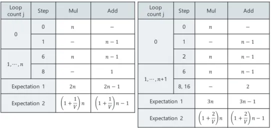
Table 1 summarizes the number of multiplications (Mul) and additions (Add) executed at each step in the j-th loop of SDPS (left) and SDRT (right). Each table has an entry,

Expectation 1, which presents the expected number of operations computed with the probability derived in 6.1.2. As an example, the average number of multiplications in SDPS is computed as

n

X

j=1

p_j·(1+j)n

=n+n

n−1

X

j=1

pj·j

=n+n











1−2a+2a





 1−₁

N

n

1− ¹

N

















≈2n.

This result implies that the algorithm halts mostly at the first loop ifNis sufficiently large. In other words, the probability that the algorithm is continued after the first loop is negligibly small. The worst-case complexity is no more thanO(n²), which occurs when the sign is not determined until the last loop.

The standard deviation for the number of multiplications is derived as

σ≈

r6a N ·n.

This represents a very steep distribution around the average.

The result in Table 1 leads to the following Theorem.

Theorem 4:

If the input to SDPS and SDRT is chosen uniformly and at random, and ifN =2^wis sufficiently larger than 1, then the expected number of operations is O(n) multiplications

andO(n) additions

Furthermore, with nmultipliers operating in parallel, the expected number of multiplications becomesO(1). Sim- ilarly, with ann-input adder, the order of additions turns into O(1). In addition, multiplication at step 0 becomes unnec- essary ifxcan be represented byξ_iinstead of{x}_B.

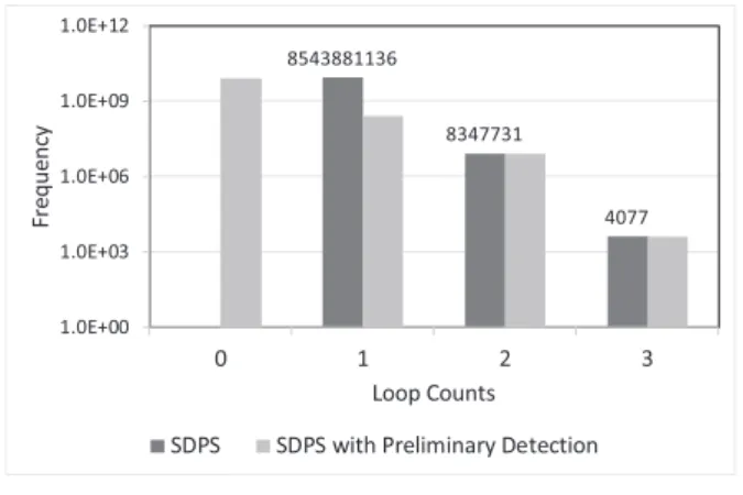
A numerical experiment was done to confirm the validity of the theoretical expression of the probability. Figure 6

(10)

Fig. 6 Frequency of loop 2.

is a histogram that shows the frequency of the loop number at which the algorithm SDPS halts when the inputxvaries from 0 to M−1. The dark gray graph is SDPS of interest here and the light gray graph will be discussed in 6.1.4. The vertical axis is shown on a log scale.

We select relatively small parameters,n =3,w =11, and (µ1, µ2, µ3)=(1,3,5), so that an exhaustive experiment onxis possible. The result agrees well with the expectation computed from the probability. In fact, the error relative to the theoretical result is less than 0.4%. The frequency of a loop count of 1 is much larger than the sum of other fre- quencies. The ratio is about (1−2a/N) : (2a/N)≈1000 : 1 both experimentally and theoretically, for our parameters. It is only nearx=0,M/2,Mthat a loop count more than 2 is seen. A similar result is obtained for SDRT.

6.1.4 Preliminary Detection for Improvement

To reduce the computation steps further, we propose to add preliminary detection steps that evaluate the first several bits of the first approximate term immediately after it is computed. Here is the pseudocode of the preliminary detection.

s1:low← hFi2^w

s2:sign←low(w−1) s3:tmp←lowVMask

s4:iftmp,Maskthen return(sign) end if

To improve SDPS, steps 2 and 3 in Fig. 2 should be replaced by the above code. In this case, symbolFat step s1 should be replaced bygx k. As for SDRT, the above code should be added immediately before step 2. This time,Fshould be replaced byh2. The constantMaskis defined as follows:

v=





 log₂







n

X

i=1

µi











 ,

Mask=2^w−1−2^v.

Maskis designed so that the MSB and vleast significant bits are zero and the other bits are one. In the preliminary detection steps,tmphas a bit string that is cut out byMask fromlow(at step s3). If the bit string is not all 1s, the sign bit is fixed and the algorithm halts. Otherwise, if the bit string is all 1s, the algorithm proceeds to compute the next term.

Let p⁰_j denote the probability that the algorithm with preliminary detection halts in the j-th loop. Then,

p⁰₀=1− 1 V, where

V =2^w−v−1. The rest are

p⁰₁= 1 V −2a

N,

p⁰_j=pj(for 2≤ j≤n).

pjis the probability defined in 6.1.2. The expectation computed using p⁰_j is shown in Expectation 2 of Table 1. The experimental result for SDPS with preliminary detection is shown in the light gray graph in Fig. 6.

6.1.5 Optimality

We next discuss the optimality of our algorithm in terms of computational complexity. According to Theorem S ([7], p.291), we must use all elements of{x}Bto compute a correct sign. Suppose we use an arbitrary binary operation that has two inputs and one output, a typical example of which is multiplication or addition. Since {x}_B hasn elements, at least (n−1) operations are necessary to obtain an output that depends on all the elements. Therefore, the number of operations for sign detection cannot be less than (n−1). In Table 1, Expectation 2 for multiplication is slightly greater thann. This shows that our algorithms are very nearly opti- mal.

6.2 Size of Lookup Table

We evaluate the memory size for a lookup table including a constant{W}_B. LetS_GandS_Hdenote the memory sizes for SDPS and SDRT, respectively. Then,

S_G=n(n+1)w≈(n+1) log₂M, S_H=n(n+3)w≈(n+3) log₂M

= log₂M2

w +3 log₂M (bit)

≈O

log₂M2 .

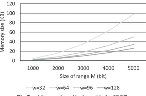
We assume here that each lookup table is a sequence of words. S_H is larger than S_G, shown in Fig. 7, with parameters w = 32, 64, 96, and 128. Even in the most memory-consuming case, w = 32, our sign detection can be implemented with 4.38 KB and 98.1 KB memories for log₂M = 1000 and 5000 bits, respectively. On the other hand, the respective memory size required by the method in [9] are more than 200 KB and 2 MB (Fig. 6(b) of [9]).

Hence, our algorithm reduces the memory size by a factor of at least 1/20 for log₂M =5000 bits. Graphs of memory

(11)

Fig. 7 Memory size of lookup table for SDRT.

size for[9]are out of the range of Fig. 7. In[9], memory size is evaluated as

O

log₂M3/(log₂log₂M)² .

Since the denominator increases very slowly, the degree of this equation in log₂M can be approximated by 3, while memory size of our algorithms is degree 2.

LetSV denote the memory size of Vu’s method[8].

Then, it follows that SV ≈n2^wlog₂nM

≈2^w











log₂M2

w + log₂n

w

! log₂M











≈O√n

M· log₂M2 .

Compared with SH, SV is about 2^w times the size. Vu’s algorithm stores all entries corresponding to all values of xi, while our algorithm stores only one representative value and produces the variation by multiplying the valueξithat depends on the value ofxi. This results in a significant memory reduction.

7. Conclusion

We have proposed efficient sign-detection algorithms, SDPS and SDRT, that compute via the Chinese remainder theorem using approximate reciprocals. The average computational complexity of the algorithms isO(n), wheren is the number of base elements. The size of lookup table is reasonably small and at most (n+3) log₂M bits. To the best of our knowledge, the proposed algorithms realize the best efficiency and the least memory. At least, they are superior to all algorithms that were evaluated in[9]. We conjec- ture that there is little hope for finding a substantially better method with an order<O(n), for the same reason as men- tioned by Knuth. The proposed algorithms make it possible to efficiently compare two integers in RNS. Now we can implement, in RNS, procedures that are important but have been circumvented due to inefficiency of comparison. Such procedures include the binary extended Euclidean algorithm and the final subtraction of Montgomery multiplication. The validity of the proposed algorithms is confirmed by computer experiment. Further study is necessary to evaluate the

proposed algorithms on FPGA or ASIC architectures.

Acknowledgments

Part of this paper is based on results obtained from a project, JPN16007, commissioned by the New Energy and Industrial Technology Development Organization (NEDO).

References

[1] L. Sousa, S. Antao, and P. Martins, “Combining residue arithmetic to design efficient cryptographic circuits and systems,” IEEE Circuit Syst. Mag., vol.16, no.4, pp.6–32, 2016.

[2] J.-C. Bajard, J. Eynard, and N. Merkiche, “Montgomery reduction within the context of residue number system arithmetic,” J. Cryptogr.

Eng., vol.8, no.3, pp.189–200, Springer, 2018.

[3] S. Kawamura, M. Koike, F. Sano, and A. Shimbo, “Cox-rower architecture for fast parallel Montgomery multiplication,” EURO- CRYPT2000, LNCS1807, pp.523–538, Springer, 2000.

[4] K. Bigou and A. Tisserand, “Improving modular inversion in RNS using the plus-minus methods,” CHES2013, LNCS8086, pp.223–

249, Springer, 2013.

[5] K. Bigou and A. Tisserand, “Binary-ternary plus-minus modular inversion in RNS,” IEEE Trans. Comput., vol.65, no.11, pp.3495–

3501, Nov. 2016.

[6] H.L. Garner, “The residue number system,” IRE Trans. Electron.

Comput., vol.EC-8, no.2, pp.140–147, 1959.

[7] D.E. Knuth, The Art of Computer Programing, vol.2, 3rd ed., Addison-Wesley, 1997.

[8] T.V. Vu, “Efficient implementations of the Chinese remainder theorem for sign detection and residue decoding,” IEEE Trans. Comput., vol.C-34, no.7, pp.646–651, July 1985.

[9] D.S. Phatak and S.D. Houston, “New distributed algorithms for fast sign detection in residue number systems (RNS),” J. Parallel Distrib.

Comput., vol.97, pp.78–95, 2016.

[10] K. Nave, A.S. Molahosseini, and M. Esmaeildoust, “How to teach residue number system to computer scientists and engineers,” IEEE Trans. Educ., vol.54, no.1, pp.156–163, Feb. 2011.

[11] S. Kumar and C.-H, Chang, “A new fast and area-efficient adder- based sign detector for RNS{2ⁿ−1,2ⁿ,2ⁿ+1},” IEEE Trans. Very Large Scale Integr. (VLSI) Syst., vol.24, no.7, pp.2608–2612, 2016.

[12] L. Sousa and P. Martins, “Sign detection and number comparison on RNS 3-moduli sets{2ⁿ−1,2ⁿ⁺^x,2ⁿ+1},” Circuits Syst. Signal Process., vol.36, no.3, pp.1224–1246, 2017.

[13] A. Hiasat, “A reverse converter and sign detectors for an extended RNS five-moduli set,” IEEE Trans. Circuits Syst. I, Reg. Papers, vol.64, no.1, pp.111–121, 2017.

[14] N. Guillermin, “A high speed coprocessor for elliptic curve scalar multiplications over Fp,” CHES2010, LNCS6225, pp.48–64, Springer, 2010.

[15] G.X. Yao, J. Fan, R.C.C. Cheung, and I. Verbauwhede, “Novel RNS parameter selection for fast modular multiplication,” IEEE Trans.

Comput., vol.63, no.8, pp.2099–2105, Aug. 2014.

[16] S. Kawamura, Y. Komano, H. Shimizu, and T. Yonemura, “RNS Montgomery reduction algorithms using quadratic residuosity,” J.

Cryptogr. Eng., vol.9, pp.313–331, Springer, 2019.

[17] G.C. Cardarilli, M. Re, R. Lajacono, and G. Ferri, “A systolic architecture for high-performance scaled residue to binary conversion,”

IEEE Trans. Circuits Syst. I, Fundam. Theory Appl., vol.47, no.10, pp.1523–1526, 2000.

Appendix A: Proof of Theorem 1

At first, if x = 0, it follows thatG(0,d) =G(0) = 0 from

(12)

condition (iii). Theorem 1 holds in this case.

Ifx , 0, we will show thatbG(x)c = bG(x, δ)cholds for ∀x ∈ [1,M −1]. FromG(x,d) = G(x)−e(x,d) and 0≤e(x,d)≤e(d), we can derive

G(x)−e(d)≤G(x,d)≤G(x).

If we substitute the relation G(x)=hG(x)i₁+bG(x)c

= x

M +bG(x)c,

to this equation, we get the following equation.

x

M −e(d)≤G(x,d)− bG(x)c ≤ x

M (A·1)

From now on, we assumed=δ, which satisfies the assumption of Theorem 1. Under this condition, the lower bound of (A·1) is assessed as follows:

x

M −e(δ)≥ x M − 1

2M =2x−1

2M ≥ 1

2M >0. (A·2) We apply condition x ≥ 1, which comes from our tempo- ral assumption, x , 0. The upper bound of (A·1) can be evaluated as

x

M ≤ M−1

M <1. (A·3)

From (A·1)–(A·3), it follows that 0<G(x, δ)− bG(x)c<1.

This means that bG(x)c=bG(x, δ)c.

This relation justifies the equation

G(x, δ)− bG(x)c=G(x, δ)− bG(x, δ)c

=hG(x, δ)i1.

Substituting this relation andd=δto (A·1), we obtain x

M −e(δ)≤ hG(x, δ)i₁≤ x

M. (A·4)

Now, we evaluate the range ofhG(a, δ)i1using (A·4) when ais in the range of a positive number as

a∈ {x|1≤x<M/2,xis an integer}.

The lower bound on (A·4) is derived by (A·2), and the upper bound is

(upper bound)= x

M <(M/2) M = 1

2. Thus, we obtain

0<hG(a, δ)i1< 1 2.

Therefore,b−1=0 holds forhG(a, δ)i1. Similarly, if

b∈ {x|M/2<x≤M−1,xis an integer}, then

min(b)=











M/2+1, if M is even, M/2+1/2, if M is odd.

The upper bound of (A·4) is assessed by (A·3) and the lower bound of (A·4) is

(lower bound)= x

M −e(δ)≥min(b) M − 1

2M ≥1 2. Thus,

1

2 ≤ hG(b, δ)i1<1

holds. Therefore,b−1 = 1 holds forhG(b, δ)i1. Theorem 1 is proven whenx,0 as well.

(Q.E.D.) From the above discussion, when M is even, we can replace the assumption of Theorem 1, e(δ) < 1/2M, by e(δ)<1/M.

Appendix B: Upper Bound ofhigh(k)

Lemma 2 ensures thathigh(k)<2^wholds for 1≤k≤n.

Lemma 2:

If

e(n)≤ 1 2M, then for 1≤k≤n,

high(k),

















n

X

i=1

ξiµ^k_i





 w











<2^w.

Proof:

The conclusion of Lemma 2 is equivalent to

n

X

i=1

ξiµⁿ_i <2^2w (A·5)

holding whenkhas a maximum value ofn. Equation (A·5) is to be proven.

Frommi≤2^w, we obtain

n

X

i=1

ξi

2^w µi

2^w n+1

≤

n

X

i=1

ξi

m_i µi

2^w n+1

.

Since the right-hand side equalse(x,n), we obtain e(x,n)≤e(n)≤ 1

2M

from the assumption of Lemma 2. Thus,

(13)

n

X

i=1

ξ_i 2^w

µ_i 2^w

n+1

≤ 1 2M

holds. This equation can be modified as

n

X

i=1

ξ_iµⁿ_i⁺¹ ≤2⁽ⁿ⁺^2)w 2M

= 2^2w 2Qn

i=1

1− ^µⁱ

2^w

≈2^2w−1

<2^2w. (A·6)

Ifµiis a non-negative integer andnis positive integer, µⁿ_i ≤µⁿ_i⁺¹

holds. This proves (A·5).

(Q.E.D.) Lemma 3 ensures thathigh(1)<2^w−1.

Lemma 3:

If

e(n)≤ 1 2M,

then, fork=1, it holds that high(1),

















n

X

i=1

ξiµi





 w











<2^w−1.

Proof:

It suffices to show that

n

X

i=1

ξ_iµ_i<2^2w−1. (A·7)

We will assess the left-hand side by case. Supposen ≥ 2 andµ_i ,1; then 2µ_i≤µ²_i holds for anyi, even ifµ_i=0 for somei. With these in mind, we have the following cases.

Case 1:µ_i,1.

2ⁿ

n

X

i=1

ξ_iµ_i≤

n

X

i=1

ξ_iµⁿ_i⁺¹

From (A·6) of the proof of Lemma 2, the upper bound is modified as

2ⁿ

n

X

i=1

ξiµi<2^2w

n

X

i=1

ξiµi<2^2w−n

Note thatn≥2, so this equation proves (A·7).

Case 2: whenµ1=1.

2ⁿ

n

X

i=2

ξ_iµ_i+ξ₁≤

n

X

i=1

ξ_iµⁿ_i⁺¹

From (A·6) of the proof of Lemma 2, the following equation is derived.

n

X

i=2

ξ_iµ_i< 1 2ⁿ

2^2w−ξ₁

≤2^2w−n This proves (A·7) and thus Lemma 3.

(Q.E.D.) Appendix C: First and Second Entries of Reciprocal

Table

The elements of a reciprocal table,h_i(k), can be computed by the following recurrence formula, sequentially fromk= 1.

hi(k)=









 1 mi

−

k−1

X

j=1

hi(j)2^−jw





 2^wk





Substituting a power series for 1/mileads to hi(k)=









 1 2^w

∞

X

l=0

µi

2^w l

−

k−1

X

j=1

hi(j)2^−jw





 2^wk



 .

Ifk=1 and we substituteεi=µi/2^w, then hi(1)=

$ 1 1−εi

%

=

$ 1+ εi

1−εi

%

=1.

The last equation is due toε_i<1/2.

Similarly, ifk=2, we can derive hi(2)=

$

µi+ µiεi

1−ε_i

%

=µi+



 1 2^w· µ²_i

1−ε_i



.

To find the condition in which the value in the last floor symbol is less than 1, we define f as f(µi)=µ²_i +µi−2^w. The positive root of f(µi)=0 is given by

s=

√

2^w⁺²+1−1

2 .

We can summarize the result as hi(2)=











µ_i, (0≤µ_i<s) µ_i+1,

s≤µ_i<2^bw/2c .

Since sis rather close to 2^bw/2c, if we chooseµ_iat random, hi(2)=µiholds with a very high probability.

Appendix D: Overflow Detection of Modular Addition An overflow (OF) detection of modular addition is known as a relevant problem for sign detection. To realize an efficient OF detection, we represent an integer xby{x}_B appended withsx, a sign bit of Definition 1. As shown in Fig. A·1, the OF flag can be computed efficiently with a single call to the sign function.

(14)

Fig. A·1 Overflow detection of addition.

Shinichi Kawamura received B.E., M.E., and D.E. degrees in Electronic Engineering from the University of Tokyo in 1983, 1985, and 1996, respectively. He joined Toshiba Corpo- ration in 1985, and retired from the company in 2020 as a Senior Fellow. Currently, he is a Deputy Director of the Cyber Physical Security Research Center (CPSEC) at the National Insti- tute of Advanced Industrial Science and Tech- nology (AIST), Tokyo, Japan. His research interests are in cryptography and its application to security systems. Dr. Kawamura is a Fellow of IEICE, a Senior Member of IEEE, a Senior Member of IPSJ, and a member of IACR. He was a re- cipient of IEICE’s Young Researchers’ Award in 1993, the Distinguished Service Award from IEICE Engineering Sciences Society in 2006, and an IPSJ Specially Selected Paper Certificate in 2014.

Yuichi Komano was born in 1978. He received his M.S. and D.Sci. degrees from Waseda University in 2003 and 2007, respectively. He belongs to the Corporate R&D center of Toshiba corporation since 2003. His research interest includes the cryptography and information security. He is a senior member of the IEICE and IPSJ, and a member of the IACR, IEEE and ACM.

Hideo Shimizu was born in 1964. He received his M.E. and D.E. degrees from Kana- zawa Institute of Technology, Ishikawa, Japan, in 1990 and 1994, respectively. He joined To- shiba Corporation in 1994. From 1999 to 2000, he was a researcher at the Information & Com- munication Security Project of Telecommunica- tions Advanced Organization of Japan. He has been engaged in cryptography and information security.

Saki Osuka received the M.E. degrees from Nara Institute of Science and Technology, Nara, Japan in 2019. She is currently working to- ward the Ph.D. degree in information sciences at Nara Institute of Science and Technology, Nara, Japan. Her research interests include electro- magnetic compatibility and information security. Ms. Osuka is a member of IEEE.

Daisuke Fujimoto received B.E., M.E., and Ph.D. degree from Kobe University, Japan, in 2009, 2011 and 2014, respectively. He is currently an assistant professor in the Graduate School of Information Science, Nara Institute of Science and Technology, Nara, Japan. He is also a visiting assistant professor in the Institute of Advanced Sciences, Yokohama National Uni- versity. His research interests include hardware security and implementation of security cores.

He is a member of IEEE and IEICE.

Yuichi Hayashi received Ph.D. degree in information sciences from Tohoku University, Sendai, Japan, in 2009. He is currently a Pro- fessor of Nara Institute of Science and Tech- nology. His research interests include electro- magnetic compatibility and information security. Prof. Hayashi is the Chair of EM Infor- mation Leakage Subcommittee in IEEE EMC Technical Committee 5.

Kentaro Imafuku received his Ph.D. degree from Waseda University. After professional ex- periences in Waseda university, University of Rome Tor Vergata (JST/JSPS overseas young research fellowship), and the University of To- kyo, he is working in National Institute of Ad- vanced Industrial Science and Technology. He is conducting theoretical researches on applications of physics and information theory to computer science and engineering.