Panel Data Research Center, Keio University
PDRC Discussion Paper Series
賃金と睡眠時間
梶谷真也
2019 年 10 月 8 日
DP2019-001
https://www.pdrc.keio.ac.jp/publications/dp/5487/
Panel Data Research Center, Keio University
2-15-45 Mita, Minato-ku, Tokyo 108-8345, Japan
[email protected]
8 October, 2019
賃金と睡眠時間 梶谷真也
PDRC Keio DP2019-001 2019 年 10 月 8 日
JEL Classification: I12; J24; J31
キーワード: 労働生産性;睡眠時間;時間配分;賃金;労働時間 【要旨】 本論文では,慶應義塾大学が実施する『日本家計パネル調査:KHPS データ』の 2005 年から 2017 年までの男性回答者の情報を用いて,賃金率が睡眠時間に与える逆の因果関係を考慮しな がら,睡眠時間が賃金率に与える影響を分析する.具体的には,操作変数法を用いた固定効果 モデルの推定を行うことで,時間不変な要因・時間可変な要因の双方によって発生する内生性 を考慮する.回答者の居住地域の「月平均日照時間」と「年平均気温」を操作変数に用いて分 析した結果,週平均睡眠時間が 1 時間増加すると賃金率は約 4-6%上昇することが統計的に有 意に確認された.正規労働者に限定した場合でも,約 3-5%の賃金率の上昇が統計的に有意に 確認された.これらの結果は,睡眠時間の増加が労働生産性を上昇させることを示している. また,内生性を考慮しない場合(固定効果モデル)では,係数値に負のバイアスが生じている ことが分かった.このことは,賃金率の増加が睡眠時間を減少させるという逆の因果関係が存 在していることを示唆している. 梶谷真也 京都産業大学 経済学部 〒603-8555 京都府京都市北区上賀茂本山 [email protected] 謝辞:本研究は科研費 若手研究(B)「個人の時間配分と生産性・健康資本の格差」 (15K17080)による研究成果である。ここに記して謝意を表したい。
Return to Sleep
Shinya Kajitani
∗October, 2019
Abstract
Most people spend a substantial amount of time sleeping. I examine the causal effect of sleep on labor productivity, utilizing panel datasets for Japanese males. I deal with the potential endogeneity of the decision about how many hours to sleep by using a fixed effects model with an instrumental variables estimation technique. My findings show that a one-hour increase in weekly sleeping hours increases the wage rate by 4–6%. Sleep duration does indeed enhance labor productivity for Japanese males.
Keywords: Labor productivity, Sleep duration, Time use, Wage, Working hours. JEL Classification: I12, J24, J31.
∗Corresponding author. Associate Professor, Faculty of Economics, Kyoto Sangyo University,
Mo-toyama, Kamigamo, Kita-ku, Kyoto-city 603-8555, Japan. Phone number: +81-75-705-1739. E-mail address: [email protected]
1
Introduction
In the standard labor supply model, individuals make trade-offs between the consumption of goods and the consumption of leisure, where leisure is defined as time not spent at work. However, Juster and Stafford (1991) point out that it is essential to shed light on the productive uses of leisure rather than leisure as consumption. For example, Fahr (2005) examines the determinants of time spent on educational leisure, which means the educational character of certain leisure activities. Educational leisure has a productivity component compared with purely consumptive leisure.
Many past studies in economics suppose hours of sleep as exogenous. This is because a need for sleep is biologically determined. By contrast, when sleep is classified as a type of leisure, sleep could be regarded as productive leisure. A human spends many hours of the day on sleep, which is a physiological function to recover from cerebral fatigue. Medical studies indicate that sleep plays an essential role in influencing labor productivity. Horne (1988) points out that the organ most affected by sleep loss is the cerebrum. When the human experiences sleep deprivation, the cerebrum requires sleep for its repair. Walker (2017) summarizes that sleep restores one’s learning ability and offers motor skill improvement while sleep deprivation causes a decline in concentration. Hafner et al. (2016) suggest that insufficient sleep is costly for employers because it reduces workplace productivity. These studies suggest that sleep also has a productivity component. When labor markets are competitive, the derivation of the labor demand schedule leads to a first-order condition for the firm that equates the wage to the marginal product of labor. In this case, the wage changes derive from labor productivity changes. If sleep enhances labor productivity, sleep could have positive effects on wages.
Individuals vary in the amount of time that they allocate to sleep. While some part of this variation is biologically determined, another part of this variation is related to choices influenced by economic incentive, as Biddle and Hamermesh (1990) point out. In their theoretical model, while sleep is a function of the individuals’ wage rate, their demand for sleep allows for the possibility that sleep enhances labor productivity. They point out that the relationship between wages and sleep could be causal in both directions.
In this study, I examine whether sleep affects productivity for Japanese male workers, using the Keio Household Panel Survey which is a nationally representative survey panel
in Japan.1 I resolve the endogeneity between wage and sleep by using the fixed effects model with an instrumental variables estimation technique. To capture a representative of individuals’ long-run time use, I focus not on the hours of sleep on the day of the interview but on the usual sleeping hours. I am interested in the sleeping time of individuals over a period of time: person-months or person-years rather than person-days. Meanwhile, my productivity measures are average hourly labor income and average hourly wages in the year of the interview.
My contribution to previous studies is twofold. First, to identify the causal relation-ship between productivity and sleep, I use a panel estimation with instrumental variables removing both time-invariant and time-variant unobserved heterogeneities among work-ers. Locations further east will experience an earlier average sunset than areas further west in the same time zone. When sunset occurs at an early hour, individuals tend to fall asleep earlier on condition that there is no artificial light exposure (Walker 2017). Circadian rhythms are entrained to solar cues, ensuring that behavioral, genetic, and physiologic rhythms are timed with daily changes in the environment (Czeisler and Goo-ley 2007). Because of circadian rhythms, melatonin, which induces sleep, is released after sunset. While time zone cues help to determine social scheduling such as work schedules and school start times, the social schedules are not so responsive to the solar cues, as Hamermesh et al. (2008) discuss. For example, if individuals on the late sunset side of a time zone boundary tend to go to bed at a later time, many of them cannot fully com-pensate in the morning by waking up later (Giuntella and Mazzonna 2019). Thus, sunset time can have significant effects on sleeping hours. Giuntella et al. (2017) identify the effect of sleep on cognitive skills and depression symptoms exploiting Chinese variation in average annual sunset time between cities as an instrument. Both China and Japan have a single time zone. The sunset time disparities between areas under the single time zone are informative for identifying the effects of sleep as the instrument. However, since the sunset time disparities depend entirely on longitude, average annual sunset time is time-invariant within cities. That is, the sunset time is a fixed feature of a location. This
1In Japan, women are more likely to quit their jobs after marriage and childbirth than in other
developed countries. Some women return to work after childbirth, and others do not. Besides, the distribution of average hours of work is different between males and females. Thus, working status is quite different between males and females during their careers. The analysis of sleep effects on wage for females could be a little more complicated than the analysis for males. For these reasons, the analysis in this study is restricted to Japanese males.
identification strategy did not allow me to employ a fixed effects model when I consider the time-variant unobserved heterogeneity among workers.
Instead, I exploit variation inaverage annual temperature and average annual sun-shine duration between cities as the instruments. One of the most reliable environmental timing cues that entrains the circadian rhythms is the daily temperature cycle (Buhr et al. 2010). Cable et al. (2007) outline the evidence that the circadian rhythm of core temperature is affected by ambient temperature. Rifkin et al. (2018) review numerous physiologic studies and point out that the thermal environment is a significant determi-nant of sleep quality. Frazis and Stewart (2012) point out that the instruments should predict long-term time-use, rather than short-term, when the dependent variable is a long-term outcome such as productivity or wages. Average annual temperature (average annual sunshine duration) is a general long-term indicator of the heat (cloudiness) of the location. Some studies show that there is no significant long-term relationship between climate and one’s performance or productivity (e.g., Graff Zivin et al. 2018), while there is a significant short-term relationship between climate and one’s performance or produc-tivity (e.g., Graff Zivin and Neidell 2014; Graff Zivin et al. 2018). These indicate that the regional differences in annual weather condition enable us to identify the effects of the usual sleeping hours as the instruments in the fixed effects model when considering the time-variant unobserved heterogeneity among workers.
Second, I examine the Japanese case, which is an excellent example for finding a re-lationship between hours of sleep and productivity. Japan has, indeed, been categorized in the group of OECD countries with the shortest sleeping hours. According to OECD (2009), the Japanese slept the second least in the 18 OECD countries surveyed in 2006, while the French enjoyed one hour more sleep than the Japanese. I show that sleep is a vital wage determinant in Japan and, therefore, an essential part of a Japanese individ-ual’s time-allocation decision. My empirical results should contribute to the accumulating studies on this topic.
The estimation results considering both the time-invariant and the time-variant un-observed heterogeneities showed that a one-hour increase in weekly sleeping hours for Japanese males increases both hourly labor income and hourly wage by 5–7%. In the case of regular employees, a one-hour increase in weekly hours of sleeping increases both hourly labor income and hourly wage by 3–5%. The rest of this paper is organized as follows. In Section 2, I review previous studies which document the relationship between
sleep and wage. Section 3 describes the data, and Section 4 presents the empirical frame-work. Section 5 presents and discusses the estimation results, and Section 6 concludes.
2
Previous Studies
There are several trends in sleeping hours in developed countries. Juster and Stafford (1991) examine the changes in average hours of sleep between the 1960s and 1980s and show that weekly sleeping hours decrease by 0.8 hours for males and 1 hour for females in the United States, and by 3.8 hours among men and 2.6 hours among women in Japan. Meanwhile, Gimenez-Nadal and Sevilla (2012) find that average weekly sleeping hours increase for both men and women in Canada, Finland, France, the Netherlands, and the United Kingdom from the 1970s until 2000. Kuroda (2010) points out that the United States has a slight increasing trend in sleep duration in the ten years between 1991 and 2001, although Japan has a decreasing trend in sleep duration after 1991. Basner and Dinges (2018) also show that average sleep duration in the United States increases after 2003.
When individuals get more (less) sleep, they need adjustments that allow for extended (shortened) hours of sleep while satisfying the time budget constraint. One of the modi-fications is that they increase (decrease) their sleep duration by allocating less (more) to the market sector. Some studies find that market work has a substitution relationship with sleep. Brochu et al. (2012), using Canadian time use data, and Antill´on et al. (2014), using American time use data, find that a higher unemployment rate, that is, deterioration in the economic condition, is associated with longer sleep duration. Aguiar et al. (2013), who use data from the American Time Use Survey between 2003 and 2010, examine how individuals allocate their time during a recession and show that hours of sleep increase by 1% when market work hours fall by 10%. Gimenez-Nadal and Molina (2015) examine the relationship between health status and time allocation taking into account that the more time individuals devote to another applies on time. Using time-use data in six European countries, they show that there are significant correlations between hours of paid-work and hours of sleep.
Biddle and Hamermesh (1990) is the first study to demonstrate that some variation in time spent sleeping may result from a choice in response to changing economic incen-tives. They emphasize that time spent sleeping could be affected by wages. Assuming
that sleep is an entirely time-intensive commodity whose consumption provides utility in the same way as other products do, higher wages make individuals’ sleep less because the opportunity cost of sleeping is higher. However, sleep can add to the individuals’ produc-tivity: That is, sleep has a productivity component. The idea that sleep and productivity are related is supported by evidence from some sleep-related studies. Recent studies also demonstrate that insufficient sleep is costly for employers by reducing workplace produc-tivity. For example, Hafner et al. (2016) using large-scale employer-employee datasets in the United Kingdom suggest that workers who sleep less than six hours per day report on average about a 2.4 percentage point higher productivity loss due to absenteeism or presenteeism than workers sleeping between seven to nine hours per day. Biddle and Hamermesh (1990) layout a simple model of time spent sleeping as a choice variable where demand for sleep allows for the possibility that sleep enhances labor productivity, it is also assumed to generate utility, and find that higher wages are associated with less sleep. Asgeirsdottir and Zoega (2011) extend Biddle and Hamermesh’s contribution by modeling the decision to sleep as an investment decision in the level of daytime alertness (e.g., that an individual enjoys during the day). They demonstrate that higher wages will make the worker sleep less even when assuming sleep has a positive effect on wages. These indicate that the relationship between wages and sleep could be causal in both directions.
Considering the endogeneity between wages and sleep, some previous studies examine the effect of sleep on wages. Gibson and Shrader (2018) investigate the short-run and long-run effects of sleep on wages (earnings) in the United States by exploiting variation in sunset time within US time zones. When examining the long-run effect of sleep on wages (earnings), Gibson and Shrader (2018) use average annual sunset time as an in-strument. Their identification strategy is based on the fact that locations farther east experience earlier average sunset than areas farther west in the same time zone. Circa-dian rhythms cause melatonin to be released after sunset, and melatonin induces sleep. As previous studies in neuroscience point out, the earlier sunset occurs, the earlier in-dividuals tend to fall asleep on condition that there is no artificial light exposure. By contrast, as Hamermesh et al. (2008) suggest, social scheduling such as work scheduling is not so responsive to solar cues. These indicate that the sunset time disparities between areas under the same time zone are informative for identifying the effects of sleep as the instrument. Gibson and Shrader (2018) demonstrate that a 1-hour increase in average
weekly sleep increases wages (earnings) by 8% (5%) in the long-run.
However, Gibson and Shrader (2018) do not examine the causal relationship between wages and sleep considering time-invariant unobserved heterogeneities among workers. The fixed effects instrumental variables (FEIV) procedure is useful to identify the causal relationship between wages and sleep removing both time-invariant and time-variant unobserved heterogeneities among workers. When using the FEIV procedure, exclusion instruments are required to be time-variant. However, because sunset time depends entirely on latitude (longitude), average annual sunset time is time-invariant within cities.
3
Empirical Framework
My identification strategy exploited the variation in average annual temperature and average annual sunshine duration between cities, while controlling for time-invariant in-dividual characteristics. I consider the following model:
ln (Wit) = α1Sleepit+ Xitα2 + uit, i = 1, . . . , N, t = 1, . . . , Ti (1)
uit= µi+ σit (2)
where Wit denotes average hourly labor income (average hourly wage) for individual i
at the time of survey t, Sleepit is the usual nighttime sleeping hours for individual i at
the time of survey t. Xit denotes a vector of time-variant control variables: Age and
Age squared, which control for age-related effects; Tenure and Tenure squared, which control for tenure-related effects; a 0–1 dummy variable Union, which takes the value one if there is a union at the respondent’s workplace and 0 otherwise. Some studies demonstrate that unions in Japan contribute to an increase in the average wage (e.g., Hara and Kawaguchi 2008). To take family structure into account, I also include a 0– 1 dummy variable Married, which takes the value one if the respondent has a spouse and zero otherwise, and Number of child under aged 6, which controls for the number of dependent children who are aged under six. N is the number of individuals and Ti is the
number of observations available for individual i indicating that I have an unbalanced panel. As equation (2) indicates, uit is an error term which consists of a time invariant
individual fixed effect µi and an idiosyncratic error σit. The coefficient α1 in equation (1)
The possibility of the endogeneity of the respondents’ hours of sleep Sleepitin equation
(1) is an obstacle to estimating the causal effect of sleep on wages. Given the discussion in Section 2, there would be a reverse causality between sleep and wages; higher wages raise the opportunity cost of sleeping time; sleep may be correlated with unobservable worker characteristics that also influence wages. To avoid this endogeneity problem, I employ the fixed effects model with an instrumental variables estimation technique. For equation (1), the FEIV procedure is to find time-variant variables that are related to an individual’s hours of sleep but are unrelated to his wages. I use an instrumental variables strategy that exploits differences in average annual temperature and average annual sunshine duration across Japanese cities as sources of exogenous variation in hours of sleep. I assume the following equation to explain an individual’s sleeping hours:
Sleepit = β1T empct+ β2Sunct+ Xitβ3+ eit, (3)
eit = µi+ ηit (4)
where T empct is the average annual temperature for city c where individual i lives at the
time of survey t, and Sunct is the average annual sunshine duration for city c where
indi-vidual i lives at the time of survey t. eitis an error term which consists of a time-invariant
individual fixed effect µi and an idiosyncratic error ηit. Frazis and Stewart (2012) point
out that the instruments should predict long-term time-use when the dependent variable is a long-term outcome such as productivity or wages. To identify the causal relation-ship between sleep and wages removing both time-variant unobserved heterogeneities, I exploit regional variation in annual weather conditions; average annual temperature, and average annual sunshine duration as the instruments. Both average annual temperature and average annual sunshine duration are general long-term climate indicators of the lo-cation. Graff Zivin et al. (2018) reveal that there is no significant long-term relationship between climate and one’s performance or productivity.
Prolonged periods of high temperatures lead to persistently high nighttime tempera-tures in the United States (Melillo et al. 2014). Buhr et al. (2010) point out that one of the most reliable environmental timing cues that entrain circadian rhythms is the daily temperature cycle. Cable et al. (2007) outline the evidence that the circadian rhythm of core temperature is affected by ambient temperature. Some physiologic studies report that human sleep is highly regulated by temperature. Obradovich et al. (2017) examine
the association between self-reported sleep and objectively measured temperature geolo-cated to the city level and show that a one-degree Celsius deviation in monthly nighttime temperature is associated with an increase of three nights of insufficient sleep per 100 individuals. Meanwhile, there is a positive relationship between sunshine duration and temperature. van den Besselaar et al. (2015) confirm a strong relationship between sun-shine duration and temperature trends over Europe since the second half of the twentieth century.
Figure 1 illustrates the annual variation in the long-term climate indicators among cities, at the nearest observatory from the KHPS respondent’s residential area. As shown in Panel A, the average temperature decreases at higher latitudes and longitudes, while there is less annual variation in average temperature within cities. By contrast, in Panel B, there is a large annual variation in average sunshine duration within cities, while average sunshine duration is relatively less associated with latitude and longitude.
[Figure 1 around here]
4
Data: Overview of the Keio Household Panel
Sur-vey
My data were drawn from Wave 1, conducted in 2004, to Wave 14, conducted in 2017, of the Keio Household Panel Survey (KHPS), which is one of the Japan Household Panel Survey (JHPS/KHPS) datasets. The first wave of the KHPS was conducted in the period of January–March 2004 with a sample size of approximately 4,000 households nationwide. To compensate for sample attrition, approximately 1,400 and 1,000 new survey house-holds were recruited in 2007 and 2012, respectively. The KHPS aims to investigate various aspects of household behavior, including time allocation and labor supply behavior. It contains information on households, families, and individuals. Because, for married cou-ples, the KHPS asks identical questions of both the respondent and his/her spouse, the first wave contains detailed data on approximately 7,000 individuals.2
The KHPS datasets, excluding 2004 and 2007, contain information on average sleep duration. Respondents are asked to report how long they sleep each day, on average.
2Detailed information on the sample design of KHPS is available in Kimura (2005) and from URL:
Using this question, I calculate a measure of weekly sleep duration in hours (hours of sleep they usually take per day ×7).3 By contrast, the KHPS asks the respondents who performed paid work or took leave from work in the month prior to the survey about the amount of pre-tax income from their main job in the previous year. The questionnaire also asks about the average weekly hours of paid work. Using this information, I calculate the hourly labor income: (the amount of pre-tax income from their main job ÷ [average weekly hours of paid work × 4 (weeks) times 12 (months)]).
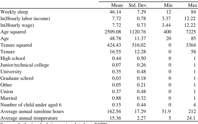
The definitions of all the variables used in the analysis in this study are summarized in Appendix Table A1. Table 1 shows descriptive statistics on all the variables used in the analysis. The sample is restricted to male individuals who meet the following three criterion: (1) the respondent performed paid work or took leave from work at the time of the survey; (2) information on all the relevant variables is available for the respondent and (3) the respondent has more than two observations (in other words, the respondent is not included in singleton groups). Appendix Table A2 indicates the effect of this criterion on the sample size available. It is noted that when the primary respondent is married and is female, the questionnaire also contains virtually identical questions to be answered by her spouse. Therefore, I include her spouse (male) in the sample used in this analysis.
[Table 1 around here]
5
Estimation Results
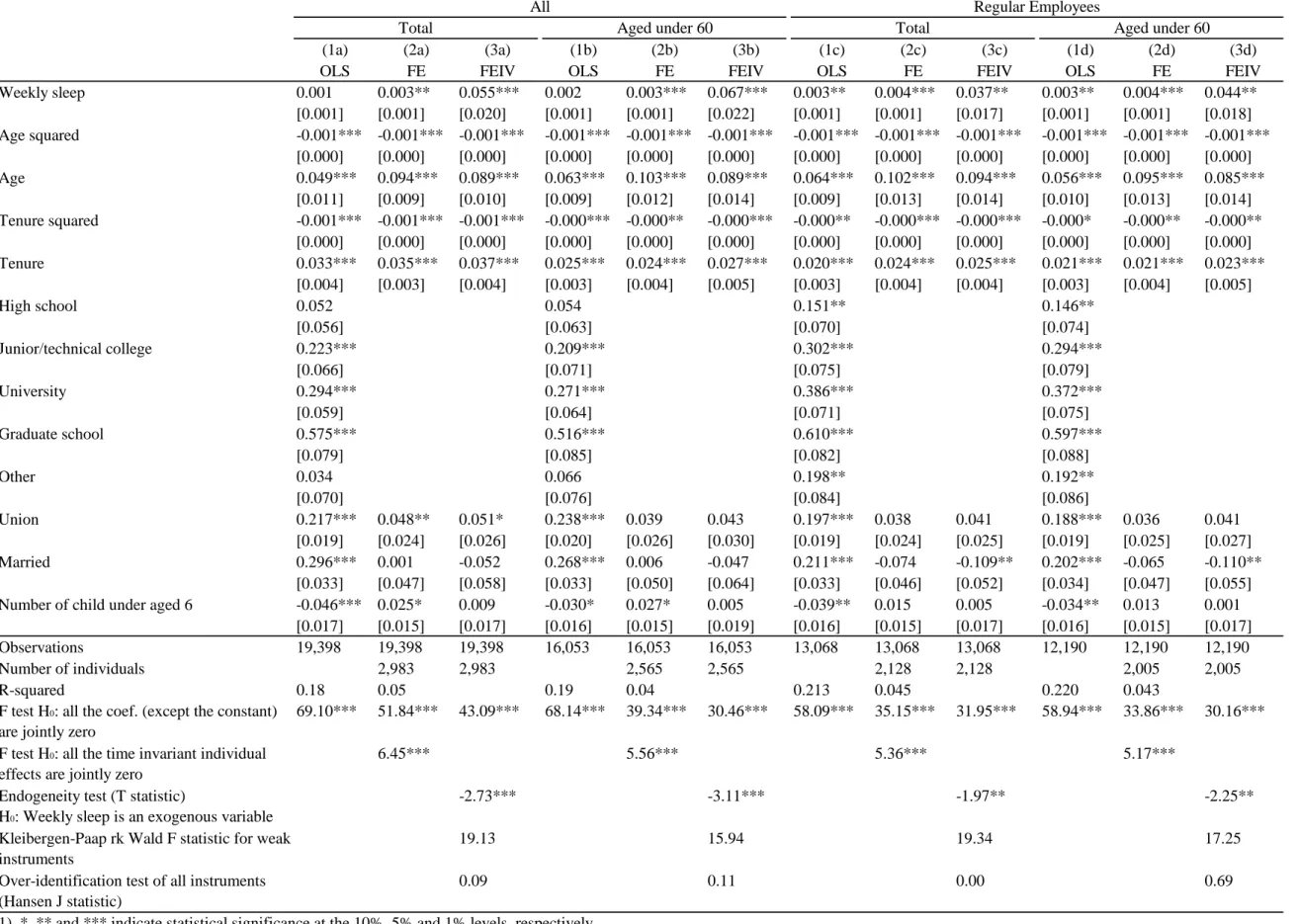
Table 2 shows the estimation results using equation (1) by an ordinary least squares (OLS) estimator that ignores both the time-invariant and the time-variant unobserved heterogeneities among individuals (Column (1)), a Fixed Effect (FE) estimator that ig-nores the time-variant unobserved heterogeneities among individuals (Column (2)) and a FEIV estimator that takes account of both the time-invariant and the time-variant unob-served heterogeneities among individuals (Column (3)). Examining the results in Column (1a), I find that, after controlling for the control variables, the estimated coefficient of Weekly sleep is insignificant. By contrast, in Column (2a), I find that, after additionally
3From 2014, the KHPS asks the respondents about their daily average sleep hours both on weekdays
and weekend days, on average. I calculate the measure of weekly sleep hours for the respondents as follows: (hours of sleep they usually take per weekday×5) + (hours of sleep they usually take per weekend
controlling for the time-invariant unobserved heterogeneities, the estimated coefficient of Weekly sleep is positive and significant. Because the results reject the null hypoth-esis that all the time invariant individual effects are jointly zero as shown in Column (2a), controlling for the time-invariant unobserved heterogeneities is required. In Col-umn (3a) where the time-variant unobserved heterogeneities are additionally controlled, the estimated coefficient of Weekly sleep is also significantly positive.
[Table 2 around here]
Examining the endogeneity test which tests the joint significance of a residual added to the model estimated by FE (see Wooldridge 2010, p. 354), as shown in Column (3a), the results reject the null hypothesis that Weekly sleep is exogenously determined. The Kleibergen-Paap rk Wald F statistic indicates that there is no problem of “weak” instruments, and an over-identification test of all instruments indicates that the FEIV estimator is to be preferred.4
It is noted that most firms set a mandatory retirement age in Japan. In the 2013 legislation, the Japanese government imposed job security for employees until the age of 65. However, most firms are not willing to extend the mandatory retirement age but are willing to re-contract at a lower wage with their “first-time retirees,” who have worked for them until mandatory retirement age.5 Most Japanese firms lower the wages
of elderly workers once they have reached their mandatory retirement age. This is very different from the case in many other countries, including the United States, where law and custom bar employers from cutting older workers’ pay and benefits when they reach a certain age. Taking a large wage reduction for these elderly employees into account, I show the estimation results excluding the individuals aged 60 and over from the sample in Columns (1b), (2b) and (3b). While the coefficient of Weekly sleep is insignificant estimated by OLS (Column (1b)), both the coefficients of Weekly sleep estimated by FE (Column (2b)) and FEIV (Column (3b)) are significantly positive.
It is noteworthy that the magnitude of the coefficient of Weekly sleep in Columns (3a) and (3b) is greater than that in Columns (2a) and (2b). This suggests that there is a
4Appendix Table A3 presents the results of the estimating equation (3). The exclusion restriction
variables are individually significant, and the null hypothesis that all the coefficients on the exclusion restriction variables are jointly zero is also rejected.
5According to the “2017 General Survey on Working Conditions (Sh¯ur¯o J¯oken S¯og¯o Ch¯osa)”
con-ducted by the Ministry of Health, Labor and Welfare, 93.4% of firms with more than 30 employees have a uniform retirement age and 79.3% of them set 60 as the retirement age.
reverse causality between sleep and wages such that a higher opportunity cost of sleeping time reduces time spent sleeping, as Biddle and Hamermesh (1990) and Asgeirsdottir and Zoega (2011) point out. An increase in the wage rate generates both income and substitution effects. The effect of the wage rate on sleep duration depends on whether the substitution effect dominates the income effect or vice versa. My estimation results demonstrate that the substitution effect may dominate the income effect.
Interestingly, when focusing only on regular employees, the difference of the coeffi-cients of Weekly sleep between Columns (3c) and (2c) is 0.033 (0.037−0.004). This value is smaller than the difference between those in Columns (3a) and (2a) (0.055− 0.003 = 0.052). As for the regular employees aged under 60, the difference value between those in Columns (3d) and (2d) (0.044− 0.004 = 0.04) is smaller than the difference value between those in Columns (3b) and (2b) (0.067− 0.003 = 0.064). These results indicate that the effect of the wage rate on hours of sleeping would be small for regular employees. Raising the opportunity cost of sleeping time could induce substitution away from sleep and towards market work: that is, hours of market work may be longer. The change in labor supply can be decomposed into two labor supply behaviors: extensive margin, indicating a worker’s entry and exit from the labor market; and intensive margin, indi-cating changes in working hours in response to a wage change. Kuroda and Yamamoto (2008) examine labor supply elasticity on intensive margins in Japan. Considering the endogeneity of wages and hours of work, they demonstrate that the labor supply elastic-ity on intensive margins is low for both males and females. One of the reasons for the low elasticity of male labor supply seems to reflect the fact that men, as regular workers, are under strong constraints of the given labor market contracts and customs. As for the regular employees, raising the opportunity cost of sleeping time may have relatively less of an effect on the substitution away from sleep and hours of market work.
Using another productivity index: the hourly wage rate, I can see that the estimated coefficients of Weekly sleep are significantly positive (Columns (a)–(d) in Table 3).6 These
results suggest that sleep duration enhances labor productivity for Japanese males. [Table 3 around here]
6While the primary respondent in the KHPS was selected by stratified two-stage random sampling,
the respondent’s spouse was not selected by random sampling. Even when I exclude the male sample who are spouses of the primary respondent from this analysis, the estimation results are similar to those shown in Tables 2 and 3. These results are available upon request.
6
Concluding Remarks
This study examined how sleep affects productivity for Japanese male workers, using the KHPS which is a nationally representative survey panel in Japan. To resolve the endo-geneity between wages and sleep due to both time-invariant and time-variant unobserved heterogeneities, I use the fixed effects model with an instrumental variables estimation technique. I focus on usual sleeping hours, which is a representative of individuals’ long-run time use and average hourly labor income (average hourly wage) as productivity measures for workers.
It is found that a one-hour increase in weekly sleeping hours for Japanese males increased both hourly labor income and hourly wage by 5–7%. This finding is consistent with Gibson and Shrader (2018) that a 1-hour increase in average weekly sleep increases wages and earnings by 5–8% in the long-run. Besides, as for regular Japanese employees, a one-hour increase in weekly hours of sleeping increased both hourly labor income and hourly wage by 3–5%. Thus, sleep duration does indeed enhance labor productivity for Japanese males.
Acknowledgements
I would like to grateful to Miki Kohara, Colin McKenzie, Haruko Noguchi and Isamu Yamamoto for their extremely constructive and helpful comments. I also would like to thank Junya Hamaaki, Charles Yuji Horioka, Wataru Kureishi, Yoko Niimi, Kei Sakata, Midori Wakabayashi, and participants at the annual meeting on Japanese Economic As-sociation 2017 Spring Meeting (Ritsumeikan University) and the 15th Annual Conference of Japan Health Economics Association (The International University of Health and Wel-fare) for their helpful comments. This study used data from the Japan Household Panel Survey(JHPS/KHPS), conducted by the Panel Data Research Center at Keio University. This study is supported by JSPS KAKENHI Grant Number 15K17080 for a project on “Allocation of Time, Health Disparity and Inequality in Productivity.”
References
Aguiar, M., E. Hurst, and L. Karabarbounis (2013) “Time Use During the Great Reces-sion,” The American Economic Review 103(5), pp. 1664–1696.
Antill´on, M., D. S. Lauderdale, and J. Mullahy (2014) “Sleep Behavior and Unemploy-ment Conditions,” Economics and Human Biology 14, pp. 22–32.
Asgeirsdottir, T. L., and G. Zoega (2011) “On the Economics of Sleeping,” Mind & Society 10(2), pp. 149–164.
Basner, M. and D. F. Dinges (2018) “Sleep Duration in the United States 2003–2016: First Signs of Success in the Fight against Sleep Deficiency?” Sleep 41(4). DOI https://doi.org/10.1093/sleep/zsy012
Biddle, J. E. and D. S. Hamermesh (1990) “Sleep and the Allocation of Time,” Journal of Political Economy 98(5), pp. 922–943.
Brochu, P, C. D. Armstrong, and L. P. Morin (2012) “The ‘Trendiness’ of Sleep: an Empirical Investigation into the Cyclical Nature of Sleep Time,” Empirical Economics 43(2), pp. 891–913.
Buhr, E. D, S. H. Yoo, and J. S. Takahashi (2010) “Temperature as a Universal Resetting Cue for Mammalian Circadian Oscillators,” Science 330(6002), pp. 379–385.
Cable, N. T., B. Drust, and W. A. (2007) “The Impact of Altered Climatic Conditions and Altitude on Circadian Physiology,” Physiology & behavior 90(2-3), pp. 267–273. Czeisler, C. A., and J. J. Gooley (2007) “Sleep and circadian rhythms in humans,” Cold
Spring Harbor Symposia on Quantitative Biology 72, pp. 579–597.
Fahr, R. (2005) “Loafing or Learning?—the Demand for Informal Education,” European Economic Review 49(1), pp. 75–98.
Frazis H. and J. Stewart (2012) “How to Think about Time-Use Data: What Inferences Can We Make about Long- and Short-Run Time Use from Time Diaries?,” Annals of Economics and Statistics 105/106, pp. 231–245.
Gibson, M. and J. Shrader (2018) “Time Use and the Labor Market: The Returns to Sleep,” The Review of Economics and Statistics 100(5), pp. 783–798.
Gimenez-Nadal, J. I. and A. Sevilla (2012) “Trends in Time Allocation: A Cross-County Analysis,” European Economic Review 56, pp. 1338–1359.
Gimenez-Nadal, J. I. and J. A. Molina (2015) “Health Status and the Allocation of Time: Cross-country evidence from Europe,” Economic Modelling 46, pp. 188–203.
Giuntella O., W. Han, and F. Mazzonna (2017) “Circadian Rhythms, Sleep and Cognitive Skills: Evidence From an Unsleeping Giant,” Demography 54, pp. 1715–1742.
Giuntella O. and F. Mazzonna (2019) “Sunset Time and the Economic Effects of Social Jetlag: Evidence from US Time Zone Borders,” Journal of Health Economics 65, pp. 210–226.
Graff Zivin J., S. M. Hsiang, and M. Neidell (2018) “Temperature and Human Capital in the Short and Long Run,” Journal of the Association of Environmental and Resource Economists 5(1), pp. 77–105.
Graff Zivin J. and M. Neidell (2014) “Temperature and the Allocation of Time: Impli-cations for Climate Change,” Journal of Labor Economics 32(1), pp. 1–26.
Hafner, M., M. Stepanek, J. Taylor, W. M. Troxel, and C. V. Stolk (2016) Why Sleep Mat-ters—The Economic Costs of Insufficient Sleep: A Cross-Country Comparative Anal-ysis, RAND Corporation. https://www.rand.org/pubs/research reports/RR1791.html Hamermesh, D. S. and G. A. Pfann (2005) “Introduction: Time-Use Data in Economics,”
Hamermesh, D. S., C. K. Myers, and M. L. Pocock (2008) “Cues for Timing and Coordi-nation: Latitude, Letterman, and Longitude,” Journal if Labor Economics 26(2), pp. 223–246.
Hara, H. and D. Kawaguchi (2008) “The Union Wage Effect in Japan,” Industrial Rela-tions: A Journal of Economy and Society 47(4), pp. 569–590.
Horne, J. (1988) Why We Sleep: The Functions of Sleep in Humans and Other Mammals Oxford University Press.
Juster, F. T. and F. P. Stafford (1991) “The Allocation of Time: Empirical Findings, Behavioral Models, and Problems of Measurement,” Journal of Economic Literature 29(2), pp. 471–522.
Kimura, M. (2005) “Design and sample characteristics of the 2004 Keio Household Panel Survey (KHPS),” in Y. Higuchi (Ed.), Dynamism of Household Behavior in Japan [I], Ch. 1. Tokyo: Keio University Press.
Kuroda, S. and I. Yamamoto (2008) “Estimating Frisch Labor Supply Elasticity in Japan,” Journal of the Japanese and International Economies 22(4), pp. 566–585. Kuroda, S. (2010) “Do Japanese Work Shorter Hours than Before? Measuring Trends
in Market Work and Leisure using 1976–2006 Japanese Time-Use Survey,” Journal of the Japanese and International Economies 24(4), pp. 481–502.
Melillo, J. M., T.C. Richmond, and G. W. Yohe, Eds. (2014) Climate Change Impacts in the United States: The Third National Climate Assessment U.S. Global Change Research Program 841 doi:10.7930/J0Z31WJ2.
Obradovich, N., R. Migliorini, S. C. Mednick, and J. H. Fowler (2017) “Nighttime Tem-perature and Human Sleep Loss in a Changing Climate,” Science advances 3(5), e1601555.
OECD (2009) Society at a Glance 2009: OECD Social Indicators OECD Publishing, Paris, Available at the following URL: https://doi.org/10.1787/soc glance-2008-en. Rifkin, D. I., M. W. Long, and M. J. Perry (2018) “Climate Change and Sleep: A
System-atic Review of the Literature and Conceptual Framework,” Sleep Medicine Reviews, 42, pp. 3–9.
van den Besselaar, E. J. M., A. Sanchez‐ Lorenzo, M. Wild, A. M. G. Klein Tank, and A. T. J. de Laat (2015) “Relationship between Sunshine Duration and Temperature
Trends across Europe since the Second Half of the Twentieth Century,” Journal of Geophysical Research: Atmospheres 120(20), pp. 10–823.
Wooldridge, J. M. (2010) Econometric Analysis of Cross Section and Panel Data 2nd Edition. MIT Press.
[Appendix Table A1 around here] [Appendix Table A2 around here] [Appendix Table A3 around here]
Figure 1: Annual Variation in the Long-term Climate Indicators among Cities
Panel A: Average Annual Temperature Disparities (degrees C)
Panel B: Average Annual Sunshine Duration Disparities (hours)
0 5 10 15 20 25 125 130 135 140 145 T em p er at u re ( d eg rees C ) East longitude 2005 2008 2011 2014 2017 0 5 10 15 20 25 25 30 35 40 45 T em p er at u re ( d eg rees C ) North latitude 2005 2008 2011 2014 2017 0 50 100 150 200 250 125 130 135 140 145 S uns hi ne dur at ion ( hour s) East longitude 2005 2008 2011 2014 2017 0 50 100 150 200 250 25 30 35 40 45 S uns hi ne dur at ion ( hour s) North latitude 2005 2008 2011 2014 2017
Table 1: Descriptive Statistics
Mean Std. Dev. Min Max
Weekly sleep 46.14 7.29 12 84
ln(Hourly labor income) 7.72 0.78 3.37 12.22 ln(Hourly wage) 7.72 0.73 3.44 12.22 Age squared 2509.08 1120.76 400 7225 Age 48.78 11.37 20 85 Tenure squared 424.43 516.02 0 3364 Tenure 16.55 12.28 0 58 High school 0.44 0.50 0 1 Junior/technical college 0.07 0.26 0 1 University 0.35 0.48 0 1 Graduate school 0.03 0.18 0 1 Other 0.05 0.21 0 1 Union 0.37 0.48 0 1 Married 0.88 0.32 0 1
Number of child under aged 6 0.15 0.44 0 4 Average annual sunshine hours 162.56 17.29 51.9 212 Average annual temperature 15.36 2.27 5 24.1 Source: Author's calculations using data from KHPS
Table 2: The Effects of Sleep on Hourly Labor Income
(1a) (2a) (3a) (1b) (2b) (3b) (1c) (2c) (3c) (1d) (2d) (3d) OLS FE FEIV OLS FE FEIV OLS FE FEIV OLS FE FEIV Weekly sleep 0.001 0.003** 0.055*** 0.002 0.003*** 0.067*** 0.003** 0.004*** 0.037** 0.003** 0.004*** 0.044** [0.001] [0.001] [0.020] [0.001] [0.001] [0.022] [0.001] [0.001] [0.017] [0.001] [0.001] [0.018] Age squared -0.001*** -0.001*** -0.001*** -0.001*** -0.001*** -0.001*** -0.001*** -0.001*** -0.001*** -0.001*** -0.001*** -0.001*** [0.000] [0.000] [0.000] [0.000] [0.000] [0.000] [0.000] [0.000] [0.000] [0.000] [0.000] [0.000] Age 0.049*** 0.094*** 0.089*** 0.063*** 0.103*** 0.089*** 0.064*** 0.102*** 0.094*** 0.056*** 0.095*** 0.085*** [0.011] [0.009] [0.010] [0.009] [0.012] [0.014] [0.009] [0.013] [0.014] [0.010] [0.013] [0.014] Tenure squared -0.001*** -0.001*** -0.001*** -0.000*** -0.000** -0.000*** -0.000** -0.000*** -0.000*** -0.000* -0.000** -0.000** [0.000] [0.000] [0.000] [0.000] [0.000] [0.000] [0.000] [0.000] [0.000] [0.000] [0.000] [0.000] Tenure 0.033*** 0.035*** 0.037*** 0.025*** 0.024*** 0.027*** 0.020*** 0.024*** 0.025*** 0.021*** 0.021*** 0.023*** [0.004] [0.003] [0.004] [0.003] [0.004] [0.005] [0.003] [0.004] [0.004] [0.003] [0.004] [0.005] High school 0.052 0.054 0.151** 0.146** [0.056] [0.063] [0.070] [0.074] Junior/technical college 0.223*** 0.209*** 0.302*** 0.294*** [0.066] [0.071] [0.075] [0.079] University 0.294*** 0.271*** 0.386*** 0.372*** [0.059] [0.064] [0.071] [0.075] Graduate school 0.575*** 0.516*** 0.610*** 0.597*** [0.079] [0.085] [0.082] [0.088] Other 0.034 0.066 0.198** 0.192** [0.070] [0.076] [0.084] [0.086] Union 0.217*** 0.048** 0.051* 0.238*** 0.039 0.043 0.197*** 0.038 0.041 0.188*** 0.036 0.041 [0.019] [0.024] [0.026] [0.020] [0.026] [0.030] [0.019] [0.024] [0.025] [0.019] [0.025] [0.027] Married 0.296*** 0.001 -0.052 0.268*** 0.006 -0.047 0.211*** -0.074 -0.109** 0.202*** -0.065 -0.110** [0.033] [0.047] [0.058] [0.033] [0.050] [0.064] [0.033] [0.046] [0.052] [0.034] [0.047] [0.055] Number of child under aged 6 -0.046*** 0.025* 0.009 -0.030* 0.027* 0.005 -0.039** 0.015 0.005 -0.034** 0.013 0.001
[0.017] [0.015] [0.017] [0.016] [0.015] [0.019] [0.016] [0.015] [0.017] [0.016] [0.015] [0.017] Observations 19,398 19,398 19,398 16,053 16,053 16,053 13,068 13,068 13,068 12,190 12,190 12,190 Number of individuals 2,983 2,983 2,565 2,565 2,128 2,128 2,005 2,005
R-squared 0.18 0.05 0.19 0.04 0.213 0.045 0.220 0.043
F test H0: all the coef. (except the constant)
are jointly zero
69.10*** 51.84*** 43.09*** 68.14*** 39.34*** 30.46*** 58.09*** 35.15*** 31.95*** 58.94*** 33.86*** 30.16***
F test H0: all the time invariant individual
effects are jointly zero
6.45*** 5.56*** 5.36*** 5.17***
Endogeneity test (T statistic)
H0: Weekly sleep is an exogenous variable
-2.73*** -3.11*** -1.97** -2.25**
Kleibergen-Paap rk Wald F statistic for weak instruments
19.13 15.94 19.34 17.25
Over-identification test of all instruments (Hansen J statistic)
0.09 0.11 0.00 0.69
All Regular Employees
1) *, ** and *** indicate statistical significance at the 10%, 5% and 1% levels, respectively.
2) Figures reported in square brackets are robust standard errors adjusted for clustering. The Kleibergen-Paap rk Wald F statistic reported is computed using the "xtivreg2" command in STATA 15. Total Aged under 60 Total Aged under 60
Table3: The Effects of Sleep on Hourly Wage
Total Aged under
60 Total
Aged under 60 (a) (b) (c) (d) FEIV FEIV FEIV FEIV Weekly sleep 0.059*** 0.066*** 0.043** 0.049*** [0.020] [0.022] [0.017] [0.018] Age squared -0.001*** -0.001*** -0.001*** -0.001*** [0.000] [0.000] [0.000] [0.000] Age 0.087*** 0.089*** 0.090*** 0.080*** [0.010] [0.014] [0.013] [0.014] Tenure squared -0.000*** -0.000 -0.000** -0.000 [0.000] [0.000] [0.000] [0.000] Tenure 0.024*** 0.016*** 0.018*** 0.016*** [0.003] [0.004] [0.004] [0.004] Union 0.041* 0.050* 0.032 0.039 [0.024] [0.026] [0.024] [0.026] Married -0.097* -0.100* -0.109** -0.110** [0.051] [0.055] [0.051] [0.054] Number of child under aged 6 -0.009 -0.010 -0.007 -0.010
[0.017] [0.018] [0.017] [0.018] Observations 19,398 16,053 13,068 12,190 Number of individuals 2,983 2,565 2,128 2,005 F test H0: all the coef. are jointly zero 30.85*** 24.36*** 27.12*** 24.77***
Kleibergen-Paap rk Wald F statistic for weak instruments
19.13 15.94 19.34 17.25
Overidentification test of all instruments (Hansen J statistic)
0.41 0.02 0.00 0.75
1) *, ** and *** indicate statistical significance at the 10%, 5% and 1% levels, respectively.
2) Figures reported in square brackets are robust standard errors adjusted for clustering. The Kleibergen-Paap rk Wald F statistic reported is computed using the "xtivreg2" command in STATA 15.
Appendix Table A1: Definitions of Variables
Variables Difinition
Weekly sleep =hours of sleep the respondent usually takes per day times 7 if before Wave 10, and =(hours of sleep he usually take per weekday times 5)+(hours of sleep he usually take per weekend day times 2) if after Wave 11.
ln(Hourly labor income) =the natural logarithm of (the amount of the respondent's yearly pre-tax income from his main job divided by the total amount of hours of his paid work a year).
the total amount of hours of his paid work a year=hours of his paid work per week (including overtime) times 4 weeks times 12 months.
ln(Hourly wage) =the natural logarithm of (the amount of the respondent's monthly salary
divided by the total amount of hours of his paid work a month) if his
compensation type is monthly salary, =the natural logarithm of (the amount of his weekly salary divided by the total amount of hours of his paid work a week) if his compensation type is weekly salary, =the natural logarithm of (the amount of his daily wage divided by the total amount of hours of his paid work a day) if his compensation type is daily wage, =the natural logarithm of (the amount of his hourly wage) if his compensation type is hourly wage, and =the natural logarithm of (the amount of his annual salary divided by the total amount of hours of his paid work) if his compensation type is annual salary, respectively. Age Respondent's age in years at the time of the survey
Tenure When the respondent answer the KHPS questionnaire for the first time: =(each year minus year when the respondent started working at his present company or organization)
When he answer it after second time: =(each year minus year when he started working at his present company or organization plus 1) if he was working at the same company or organization as 1 year ago, and =0.5 if he was at a different company or organization from 1 year ago or he was newly employed during the past year.
The respondent's highest level of educational background
(benchmark=Junior high school)
High school =1 if he completed high school, and 0 otherwise.
Junior/technical college =1 if he completed junior or technical college, and 0 otherwise. University =1 if he completed university, and 0 otherwise.
Graduate school =1 if he completed graduate school, and 0 otherwise. Other =1 if he completed other school, and 0 otherwise.
Union =1 if there is a union at the respondent's workplace, and 0 otherwise. Number of child under aged 6 The number of the respondents' children who are aged under 6. Married =1 if the respondent has a spouse, =0 otherwise.
Average annual temperature =(the summation of monthly average temperature at the nearest observatory from the respondent's residential area) divided by 12. The observatory data is provided by Japan Meteorological Agency.
Average annual sunshine duration =(the summation of sunshine hours in the month at the nearest observatory from the respondent's residential area) divided by 12. The observatory data is provided by Japan Meteorological Agency. Sunshine hours is defined as the hours during which direct solar irradiance
Appendix Table A2: Effect of Selection Criterion on Sample Sizes Original Number of respondents (Males) Eliminating observations where the respondent performed paid work or took leave from work at the time of the Wave
Original Number of spouse of the respondents (Males) Eliminating observations where the respondent performed paid work or took leave from work at the time of the Wave
Original Number of spouse of the respondents (Males) Eliminating observations where the respondent performed paid work or took leave from work at the time of the Wave
Eliminating observations where the relevant information was not available Eliminating singleton groups (groups
with only one observation) Wave 1 2,000 1,724 1,422 1,225 3,422 2,949 0 0 Wave 2 1,650 1,428 1,215 1,045 2,865 2,473 1,672 1,416 Wave 3 1,436 1,233 1,072 912 2,508 2,145 1,542 1,478 Wave 4 1,944 1,696 1,555 1,324 3,499 3,020 0 0 Wave 5 1,759 1,511 1,421 1,185 3,180 2,696 1,972 1,897 Wave 6 1,636 1,392 1,310 1,075 2,946 2,467 1,832 1,806 Wave 7 1,528 1,272 1,250 1,018 2,778 2,290 1,667 1,659 Wave 8 1,444 1,181 1,188 947 2,632 2,128 1,539 1,534 Wave 9 1,866 1,546 1,485 1,213 3,351 2,759 1,954 1,850 Wave 10 1,734 1,439 1,357 1,086 3,091 2,525 1,735 1,714 Wave 11 1,613 1,316 1,260 1,002 2,873 2,318 1,663 1,656 Wave 12 1,522 1,236 1,166 932 2,688 2,168 1,570 1,564 Wave 13 1,436 1,151 1,102 868 2,538 2,019 1,477 1,470 Wave 14 1,331 1,068 996 793 2,327 1,861 1,364 1,354 Total 22,899 19,193 17,799 14,625 40,698 33,818 19,987 19,398
Appendix Table A3: Check of the Exclusion Restriction Instrumental Variables (Fixed Effect Model)
Total Aged under
60 Total
Aged under 60 (a) (b) (c) (d) Average annual temperature -0.258*** -0.255*** -0.287** -0.224**
[0.096] [0.098] [0.125] [0.113] Average annual sunshine hours -0.021*** -0.020*** -0.026*** -0.025***
[0.004] [0.004] [0.004] [0.005] Observations 19,398 16,053 13,068 12,190 Number of individuals 2,983 2,565 2,128 2,005 F test H0: all the coef. are jointly zero 18.43*** 11.95*** 12.08*** 10.93***
F test H0: all the coef. on the exclusion restriction
are jointly zero
19.13*** 15.94*** 19.34*** 17.25***
2) Figures reported in square brackets are robust standard errors adjusted for clustering. 3) The coefficients of the other explanatory variables are not reported.
All Regular Employees