Computational Geometry and Linear Programming(Computational Geometry and Discrete Geometry)

Computational Geometry and

Linear

Programming

Hiroshi

Imai*

Department of Information Science

University

of

Tokyo

Abstract

Computational geometry has developed many efficient algorithms for geometric problems in

lowdimensions byconsidering the problems from the unified viewpoint ofgeometricalgorithms.

Itis often thecasethat such geometric problems may be regardedasspecialcasesof

mathemat-ical programming problemsin high dimensions. Ofcourse, computational-geometric algorithms

are much moreefficient than general algorithms formathematical programming when applied

to the problems in low dimensions. For example, a linear programming problem in a fixed

dimensioncan be solvedin linear time, while, for a general linear programming problem, only

weakly polynomial time algorithmsare known. Althoughnot so muchattention has been paid

to combine techniques in computational geometry and those in mathematical programming,

both of themshould beinvestigated morefromeach side infuture.

In thispaper,we first survey many usefulresults forlinearprogramming in computational

geometry suchasthe prune-and-search paradigm andrandomization and those in mathematical

$])rogralnIni_{I}\downarrow gsuc]_{l}$ as the interior-point metbod. We also demonstrate bow computational

ge-ometry and mathematicalprogrammingmay be combined for several geometric problemsinlow

and high dimensions. Efficient sequential as well as parallel geometric algorithms are touched

upon.

1

Introduction

Linearprogrammingis an optimization problemwhichminimizes alinear objective function under

linear inequality constraints:

$\min c^{T}x$

$s.t$

.

$Ax\geq b$

where$c,$$x\in R^{d},$ $b\in R^{n},$ $A\in R^{nxd},$$A,$ $b,$ $c$are given and elements $x_{I},$$\ldots$,$x_{d}$ of$x$ are $d$variables.

Linearprogramming would be the bestoptimizationparadigm that is utilized inreal applications,

since itcanbe usedas apowerful model of various discrete aswellas continuoussystems andevena

large-scale linear programming problem with thousands ofvariablesor more maybe solvedwithin

a reasonable time.

Wide applicability of linearprogramming makes it very interesting to investigate algorithms for

linearprogramming in the field of computer science. From the viewpoint oftheory of algorithms,

linearprogramuning has many fertile aspects as follows.

First, linear programming can be viewed as both of discrete optimization and continuous

op-timization. In its original formulation,the problem is a continuous optimization problem. On the

other hand, by investigating the feasible region $\{x Ax\geq b\}$, which is a convex polyhedron, it

isseen that there exists an optimum solution whichis an extreme point ofthe convex polyhedron

all the extreme points of the convex polyhedron in the worst case. Since the number

pointsmaybeexponential, thesimplex methodis regarded as a non-polynomialmethod in general.

However, in 1979, Khachian [18] showed that linear programming is polynomial-time solvable by

using anellipsoid method. Furthermore,in mid $1980’ s$_, Karmarkar [16] proposedan interior-point

method forlinear programming, which has better polynomial-time complexityinthe worstcase and

may run faster onthe average. Unlikethesimplexmethod whichtraversesapathon the boundary

of the convexpolyhedron, the interior-pointmethod works in theinteriorof the polyhedron. Since

the interiorof the polyhedron has continuous structure in itself, the interior-point method may be

saidto be an algorithm based on the continuousstructure of linear programming.

Third, linear programming is still not known to admit any strongly polynomial-time

algo-rithm. Khachian’s ellipsoid method as well as Karmarkar’s interior-point method yields weakly

polynomial-timealgorithms bynaturesince both are basedon Khachian’s ingenious approximation

idea ofsolving a discrete problem by a continuous approach. For network flow problems, which

form a useful subclass of linearprogramming, strongly polynomial-time algorithms are already

de-veloped (e.g., [25]), and this issue has been a big open problem conceming thecomplexity oflinear

programming.

Fourth, insome applications such as computergraphics, there arise linear programniing

prob-lemssuch that $d$ismuchsmaller than$n$or $d$is aconstant,say three. Thistype of linear

program-ming problems may be treated in computational geometry. Computational geometry, whose name

was christened by Shamos in mid $1970’ s[27]$, is a field in computer science which treats geometric

problemsin a unified way from the viewpoint ofalgorithms. Efficient $algorith_{1}us$ to construct the

convexhull,Voronoidiagram, arrangement,etc., have been developedas huitfulresultsof the field.

Untilnow, computational geometry has laid emphasis on low-dimensional geometric problems,

es-pecially problems in the two- or three-dimensional space. Also, most of computational geometric

algorithms are discrete ones. Computational geometry from now should tackle higher dimensional

problems and adopt more continuous approaches. One of useful techniques which computational

geometry is nowusing and somehow hasconnection continuous structure is randomization. This

in-troduces probabilistic behavior in algorithms, and to analyze such randomized algorithms we need

to treat geometric problems in a more general setting. For linear programming, computational

geometryyields a linear-time algorithm when the dimension is regarded as a constant. To derive

such an algorithm, the prune-and-search paradigm is used. This paradigm was originally used in

obtaining a linear-time algorithm for selection. Through computational geometry, the

prune-and-search paradigm is generalized to higher dimensionalproblems, and, besides linear programming,

produces manyuseful algorithms.

In this paper, wediscuss

some

of the above-mentioned results concerning linear programming.

This is done from the viewpoint of the author, and hence topics treated here might be biased

comparedwith the too general title of this paper. Through highlighting such results, whichwould

be of practical importance by themselves, we try to give some idea on future research directions

in the related fields. Although, up to herein this introduction, linearprogramming is emphasized

from the viewpoint of mathematical programming, computational geometry will also be treated as

a big subject ofthis paper. We first describe the prune-and-search paradigm and its applications

methodforlinear programming in mathematical programming insection3. In section4, combining

two paradigms in computational geometry andmathematical programming to obtain an efficient

linear programming algorithm is discussed. In fact, it is definitely useless to distinguish linear

programming in computational geometry and linear programming in mathematical programming, and we may treatand understand these problems in a more unifiedmanner.

2

Linear Programming in

Computational Geometry

In this section we first explain the prune-and-search paradigm, and its application to the

two-dimensionallinear programmingproblemin detail. Then two applications of the prune-and-search

technique tosome special linearprogramming problems are mentioned. We also describe

random-ized algorithms for linear programming.

2.1

Prune-and-search paradigm and its

application

to two-dimensional linear

programming

In many of algorithmic paradigms, given a problem, its subproblems of smaller size are solved to

obtain a solution to the whole problem. This is because the smaller the problem size is the more

easily the problem may be solved. The prune-and-search paradigm tries to reduce the problem

size by a constant factor by removing redundant elements at each stage, whose applicationto the

two-dimensional linear programming problem is describedbelow.

The prune-and-search paradigm is one of useful paradigmsin the design and analysisof

algo-rithms. It was used in linear-time selectionalgorithms [2]. As mentioned above,a keyidea of this

paradigm is to remove redundant elements by a constant factor at each iteration. In the case of

selecting the $k(=k_{0})th$ element $x$

among

$n$ elements, at the

ith

iteration, the algorithun

finds

a

subset of$s_{i}$ elements which are either all less than $x$ or all greater

than

$x$

.

Then, wemayremove

all the elements in the subset and, for $k_{i}=k_{i-1}-s_{i}$ and $k_{i-1}$ according as these elements in the

subset are less or greater than $x$, respectively, find $k$;th element

among

the remaining elements in

the next step. Roughly speaking, finding the subset of elements whose size is guaranteed to be at

least a constant factor $\alpha<1$ of the current size can be done in time linear to the current size.

Then, the total timecomplexity is bounded in magnitude by

$n+(1- \alpha)n+(1-\alpha)^{2}n+\cdots\leq\frac{1}{\alpha}n$

.

A linear-time algorithmis thus obtained.

Let

us

see how this prune-and-searchparadigm may be usedto developa linear-timealgorithm

for the two-dimensional linear programming problem,

as

shown by Megiddo [22] et al. Since this

is simple enough to describecompared with the other methods in this paper, wehere try to give

a rather complete description of this algoritlm]. A general two-dimensional linear programming

problem with$n$inequalityconstraints

can

be described as follows:

$\min c_{I}x_{1}+c_{2}x_{2}$

s.t. $a_{iI}x_{1}+a_{i2}x_{2}\geq a_{i0}$ $(i=1, \ldots,n)$

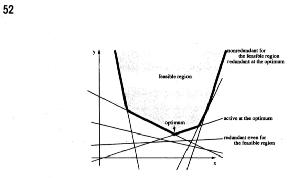
lfone can illustrate the feasible region $satis\mathfrak{g}_{r}$ing the inequality constraints in the $(x_{1}, x_{2})$-plane,

whichissimplya

convex

polygon ifbounded,the problemwouldbe veryeasytosolveillustratively (see Figure 2.1). Here,

instead

of considering the problem in this general form, we restrict our

attention to the following problem.

$\min y$

Figure 2.1. A two-dimensional linear programming problem

This is because this special problem is almost sufficient to devise a linear-time algorithm for the

generaltwo-dimensional problem, and itssimpler structure isbetter inorder toexhibitthe essence

of the prune-and-searchtechnique. Figure2.1 depicts thisrestricted problem of$n=7$

.

Weconsider the problem

as

definedabove. Define a function $f(x)$ by

$f(x)= \max\{a_{i}x+b;|i=1, \ldots,n\}$

.

Then, the problemis equivalentto minimizing$f(x)$

.

The graph of$y=f(x)$ is drawnin boldlines

in Figure

2.1.

$f(x)$ has a nice property as follows. First we review the convexityofa function. A

function$g:Rarrow R$is

convex

if

$g(\lambda x_{1}+(1-\lambda)x_{2})\leq\lambda g(x_{1})+(1-\lambda)g(x_{2})$

for any $x_{1},$ $x_{2},$$\lambda\in R$with $0<\lambda<1$

.

If the above inequality always holds strictly, $g(x)$ is called

strictly convex. Consider the problem ofminimizing a convex function $g(x)$. $x’$ is called a local

minimumsolutionif, for any sufficiently small $\epsilon>0$,

$g(x’)\leq g(x’+\epsilon)$ and $g(x’)\leq g(x’-\epsilon)$

.

$x’$is a global minimumsolutionifthe above inequality holds for arbitrary$\epsilon$. Due to the convexity,

anylocalminimum solution is a globalminimum solution. Also,if$g(x)$ is strictly convex, there is

at most oneglobalminimum solution. Suppose there is a globalminimum$x$‘ of$g(x)$

.

Given$x$, we

can determine, without knowing the specific value of$x^{*}$, which of_{$x<x^{*},$ $x=x^{*},$ $x>x^{*}$} holds by

checkingthe following conditionslocally forsufficientlysmall $\epsilon>0$:

(g1) if$g(x+\epsilon)<g(x),$ $x\leq x^{*}$;

(g2) if$g(x-\epsilon)<g(x),$ $x\geq x^{*}$;

(g3) if$g(x+\epsilon),g(x-\epsilon)\geq g(x),$ $x$is a global minimum solution.

Finally, for$k$

convex

functions_{$g_{i}(x)(i=1, \ldots , k)$},

a

function_$g(x)$ defined by

$g(x)= \max\{g_{i}(x)|i=1, \ldots , k\}$

is againconvex.

Now, retum to our problem of minimizing $f(x)= \max\{a_{i}x+b_{i}|i=1, \ldots, n\}$

.

$f(x)$ is a

continuous piecewise linear function. From the above discussions, we have the following.

(f2) Given$x$, we candetermine in which side of$x$ an optimum solution$x$“, ifit exists,lies in $O(n)$

time (first, compute $I=\{i|a_{i}x+b_{i}=f(x)\},$ $a^{+}= \max\{a_{i}|i\in I\}$ and $a^{-}= \min\{a_{i}|$

$i\in I\}$, whichcan be done in $O(n)$ time; if$a^{+}>0,$ $x^{*}\leq x$; if $a‘<0,$ $x^{*}\geq x$; if$a^{+}\geq 0$ and

$a^{-}\leq 0,$ $x$ isan optimumsolution; cf. (g1\sim 3)).

Note that this property (f2) is obtained mostly fromthe convexity of$f$

.

This property is a key in

search steps in the prune-and-search technique.

For simplicity, we assume there is a unique solution$x$“ minimizing $f(x)$ (that is, we omit the

cases where $\min f(x)$ is $-\infty$ or _{$\min f(x)$} is attained on some interval; both cases can be handled

easily byslightly changing the following algorithm). In the following, we show that

(f3) wecan find an$x$ in $O(n)$ time such that, bydetermining in which side of$x$ the minimum $x$“

lies (this can be done in $O(n)$ time from $(f2)$), wecan findat least $n/4$ constraintssuch that

a linear programming obtained by removing these constraints still has the

same

optimum

solution with the original problem (we call theseconstraints redundant).

As mentioned above, the prune-and-search techmique thus finds a constant factor of redundant

constraints,to be pruned, withrespect tothecurrent nunber ofconstraints forthetwo-dimensional

linear programming. Then, applying this recursively, we can finally remove all the redundant

constraints and get an optimumsolution in time proportional to

$n+ \frac{3}{4}n+(\frac{3}{4})^{2}n+(\frac{3}{4})^{3}n+\cdots$

which is less than $4n$

.

That is, if (f3) is true, we obtain a linear-time algorithm for this linear

programmingproblem.

To show (f3), first consider two distinct constraints$y\geq a_{i}x+b_{i}$ and $y\geq a_{j}x+b_{j}$

.

If$a_{i}=a_{j}$,

according as $b_{i}<b_{j}$ or$b_{i}\geq b_{j}$, we candiscard the ith or$j$th, respectively, constraint immediately,

because, then, $a_{i}x+b_{i}$ is smaller ornot smaller, respectively, than $a_{j}x+b_{j}$ for any $x$

.

If$a_{\mathfrak{i}}\neq a_{j}$

(suppose without loss of generality $a_{i}>a_{j}$), there exists $x_{ij}$ satisfying $a_{l}x_{ij}+b_{i}=a_{j}x_{ij}+b_{j}$

.

When$x_{ij}>x^{*}$ (resp. $x_{tj}<x^{*}$), we see the ith (resp. $jth$) constraint is redundant,since $a_{i}x^{*}+b_{i}$ is smaller (resp. greater) than $a_{j}x^{*}+b_{j}$.

Basedonthisobservation,match$n$constraints into$n/2$disjointpairs$\{(i,j)\}$, For matched pairs

with $a_{i}=a_{j}$, discard one of the two constraints according to the above procedure. For the other

pairs, compute $x_{ij}$, and find the median$x’$ among those$x_{ij}$ (recall that wecan find the median of

$n’$ numbers in _$O(n’)$ time as mentioned above) and teston which side of$x’$ the $minim\iota unx^{*}$ lies.

If$x’$ is anoptimumsolution, we have done. Otherwise, since $x’$is the median, a half of$x_{ij}’ s$ lies in

the opposite side of$x’$ with $x^{*}$. For a pair $(i,j)$ with $(x’-x^{*})(x’-x_{ij})\leq 0$, wecan determine on

which side of$x_{\mathfrak{i}j}$ the $x$

“ _{lies, and hence discard one of them as above. Thus, in $O(n)$ time, we can}

discard at least$n/4$constraints, and have shown (f3).

As noted in the discussion, even if$\min f(x)$ is $-\infty$ or is attained on some interval, we can

detectit very easilyin$O(n)$time bound. Thus, we have shown that the special linear programming

problem oftheabove-mentioned form with two variables and$n$ constraints can be solvedin $O(n)$

time. Thegeneral linear programming problem canbe solvedin linear time in an analogous way.

Still, this application of the prune-and-search paradigm to the two-dimensional linear

program-ming is quite similar to the case for linear-time selection. The prune-and-search technique can be

generalizedtohigherdimensions,and thenalgorithms obtained through it are really

computational-geometric ones. The higher-dimensional prune-and-search technique works as follows. An

under-lying assumption of the general technique is that an optimum solution is determined by at most a

constant number of the objects, which is $d$ in the nondegenerate case for linearprogranuning. In

generalterms, thealgorithmsearches relativeto$n$objectsinthe d-dimensional spaceby recursively

solving aconstant numberof sub-problemsin the $(d-1)$_-dimensionalspace recursively, thus

reduc-ing the size of the problem bya constant factor in the d-dimensional space. Roughly speaking, the

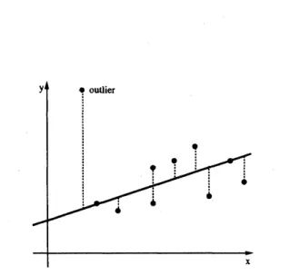
Figure 2.2. Linear $L_{1}$ approximation of points

a search relative to $n$ objects in the d-dimensional space. At eachiteration, the algorithm prunes

the remaining objects by a constant factor, $\alpha$, by applying a test a constant number of times. The

test in the d-dimensional space is an essential feature of the algorithm since the complexity of the

algorithm depends on the test being able to report the relative position ofanoptimum solution in

linear time with respect to the numberofremaining objects. The test in the d-dimensional space

is performed by solving the$(d-1)$-dimensional subproblems

as

mentioned above. Hence, thereare

a total of$O(\log n)$ steps, with the amount oftime spent at eachstep geometrically decreasing as

noted above, takinglineartime in total.

This approachwasfirst adopted by Megiddo [22] et al. By this approach, linear programming in

a fixed dimension

can

be solved

in

$o(2^{2^{d}})$ time, which is linear in$n$

.

However, this time complexity

is doubly exponentialin$d$,and the $algorit!un$may be practical only for small$d$

.

This complexity has

beenimprovedin several ways(e.g.,see[3]), butis stillexponentialwith respect to$d$

.

We will return

to this issue in the next section. Before it, we mention two applications of the prune-and-search

technique tolarger special linearprogramming problems.

2.2 Applications of the prune-and-search paradigm to special linear

program-ming

problems

Here, we mentiontwoapplications of the prune-and-searchparadigm to special linear programming

problems which are not a two-dimensional linear programming problem. One is on linear $L_{1}$

approximation of$n$points in the plane byImai, Kato and Yamamoto [12] and the other is onthe

assignmentproblem withmuch fewerdemand points than supply points by Tokuyamaand Nakano [29].

(1) Linear $L_{1}$ approximationofpoints

Approximating a set of$n$ points by a linear function, or a line in the plane, called the

line-fitting problem, is offundamental importance in numericalcomputation and statistics. The most

frequently used method is the least-squares method, but there are

alternatives

such as the $L_{1}$ and

the $L_{\infty}$ (or Chebyshev) approximation methods. Especially, the $L_{1}$ approximation is more robust

against outliers thanthe least-squaresmethod, and is preferable for noisy data.

Let $S$ be a set of $n$ points $p_{i}$ in the plane and denote the $(x, y)$-coordinate of point $p_{i}$ by

$(x_{i}, y;)(i=1, \ldots,n)$

.

For an approximate line defined by $y=ax+b$ with parameters $a$ and $b$,

the following

error

criterion, minimizing the $L_{1}$ norm, of the approximate line to the point set $S$

definesthe $L_{1}$ approximation:

$\min_{a,b}\sum_{i=1}^{n}|y_{i}-(ax_{i}+b)|$

This problemcanbeformulated as the following linear programming problem with$n+2$variables

$a,$ $b,$ $c_{i}(i=1, \ldots, n)$:

$\min$ $\sum_{i=1}^{n}c_{i}$

s.t. $y_{i}-(ax_{i}+b)\leq c_{i}$

$-y_{i}+(ax_{i}+b)\leq c_{i}$

Here, $x,,$ $y_{i}$ $(i=1, \ldots , n)$ are given constants. This linear programming problem has $n+2$

variables and more inequalities, and hence the linear-time algorithm for linear programming in a

fixeddimension cannot be applied. However,the problemis essentiallya two-dimensional problem.

Byusing the point-lineduality transformation, which is one of the besttoolsusedincomputational

geometry,we can transform this problem so that the two-diinensional prune-and-search technique

may be applied. In the $L_{1}$ approximation problem, however, any infinitesimal movement of any

point in $S$changes the

norm

(andpossibly thesolution), and, in that sense, redundantpoints with

respect to an optimum solution do not exist. Hence, direct application of the pruning technique

doesnot produce a linear-time algorithm.

Imai, Kato and Yamamoto [12] give a method of overcoming this difficulty by making full

use ofthe piecewise linearity of the $L_{1}$

norm

to obtain a linear-time algorithm. Furthennore, in

his master’s thesis, Kato generalizes this result to higher dimensional $L_{I}$ approximationproblem.

Although these algorithmsare alittle complicated, they reveal how powerful the prune-and-search

teclmique is in purely computational-geometric settings.

(2) Assignment problem

The assignment problemis a typical problemin network flow. The assignment problem with$n$

supplyvertices and fewer$k$ demand vertices isformulated as follows:

$\min$ $\sum_{i=1j}^{n}\sum_{=1}^{k}w_{ij^{X}ij}$

$s.t$

.

$\sum_{i=1}^{n}x_{ij}=n_{j}$ $(j=1, \ldots, k)$, $\sum_{i=1}^{k}x_{ij}=1$ $(i=1, \ldots, r\iota)$ $0\leq x_{ij}\leq 1$

where $x_{ij}$ are variables and $\sum_{j=1}^{k}n_{j}=n$ for positive integers $n_{j}$

.

Since this is an assignment

problem, $x_{1i}$ shouldbe an integer, but all the extreme points of the polytope of this problem are

integer-valued and hence thisproblem canbeformulated as asimple linearprogramnuing problem

of$kn$variables.

For this assignment problem, Tokuyama and Nakano [29] give the following nice geometric characterization. For this assignment problem, consider a set $S$of_$n$ points_$p$; in the k-dimensional

space whose coordinates are definedby

$p:=(w_{i1}, w_{i2}, \ldots,w_{ik})-\frac{1}{k}\sum_{j=1}^{k}w_{ij}(1,1, \ldots, 1)$

.

Each point in$S$ ison the hyperplane _{$H:x_{1}+x_{2}+\cdots+x_{k}=0$}

.

For a point $g=(g_{1},g_{2}, \ldots, g_{k})$ on

the hyperplane $H$, define

$T(g;j)= \bigcap_{h=I}^{k}$

{

$(x_{1},$

$\ldots,$$x_{k})$ onthehyperplane $H|x_{j}-x_{h}\leq g_{j}-g_{h}$

}

$T(g;j)(j=1, \ldots, k)$ partition the hyperplane $H$

.

This partition is called an optimal splitting if

candepict an example. Figure2.3 gives suchan examplewith$k=3$ and$n_{1}=n_{2}=n_{3}=5$

.

Then,

a theorem in [29] states that thereexists an optimal splitting for any $n_{j}$ satisfying the condition,

and, for the optimal splitting by$g,$ $x_{ij}$ defined by $x_{ij}=1$ if$p_{i}$ is in $T(g;j)$ and$x_{ij}=0$ otherwise

isan optimumsolutionto the

as

signmentproblem.

Thus, the assignment problem is reduced to a geometric problem of finding an optimal splitting.

Again,as in$L_{I}$linear approximation,thisproblem has$kn$variablesandmoreinequality constraints,

and the linear-time algorithm for linear programming in a fixed dimension cannot be applied.

Numata and Tokuyama [24] apply the $(k-1)$-dimensional prune-and-search technique to this

geometrically interpreted problem and obtained an$O(((k+1)!)^{2}n)$_{-time algorithm. This is linear if}

$k$ is regardedasa constant, although evenfor $k$ of moderate size the complexity becomes too big.

For $k=2,3$, this algoritinmayworkwellinpractice. A linear-time algorithm for the assignment

problemwith a constant $k$ has not been known before, and such an algorithmbecomes available

through the geometric interpretation explained above.

Besides this algorithm, Tokuyama and Nakano [29] give a randomized algorithm to solve this

problem. We willreturn to this problem at the end of the next subsection.

2.3

Randomized algorithm for linear

programming

The prune-and-search technique thus produces linear-time algorithms for linear programming in

a fixed dimension, which is theoretically best possible. However, the time complexity depends

upon the dimension $d$exponentially, and hence, even for$d$of moderatesize, the algorit!uns become

inefficient inpractice. One of ways to overcomethis difficulty is to use randomization, which has

beenrecognizedasa powerful tool incomputationalgeometry. Here, randomization does not mean

to assume any probabilistic distribution on the problem, say on the inequality constraints in this case. Instead, randomization introduces probabilistic behavior in the process of algorithms. By

randomization,it becomes possiblesomehowtoinvestigate the averagecasecomplexityof problems

besides the worst case complexity, which is quite nice from the practical point ofview. Also, it is

often thecase that randomized algorithms are rather simple and easy to implement.

Here, we first explaina randomized algorithm for linear programmingproposed byClarkson [3]

briefly. Consideratwo-dimensional linear programmingproblem treated in section2.1. Recallthat

the problem can be regarded as finding two active inequalityconstraints at an optimumsolution

andremoving all the other redundant constraints.

Take a subset $S_{0}$ of$\sqrt{n}$constraints

among

$n$constraints randomly and independently. Solve a

linearprogramming problem with this subset $S_{0}$ of constraints using the

same

objective function

to obtain anoptimum solution $(x_{0},y_{0})$ for this subproblem. In case the other$n-\sqrt{n}$constraints

are satisfied atthisoptimum solution (i.e., there is no$i$ with$y_{0}<a_{i}x_{0}+b_{\mathfrak{i}}$), this optimum solution

for the subset ofconstraints is an optimum solution for all the constraints, and we are done.

Otherwise, we compute a set $S_{1}$ of constraints $i$ which violate the computed solution: _{$y_{0}<$}

$a_{i}x_{0}+b_{i}$

.

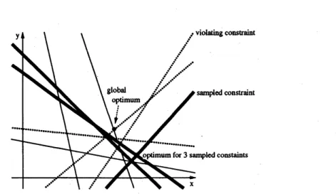
Figure2.4 illustrates thecase of$n=9$ where $\sqrt{n}=3$ constraints are randomly sampled

(denotedbyboldlines) and there areconstraints (denotedbydottedlines) violating the optimuun

Figure2.4. A randomized algorithm for linear programming

global optimuunsolution, which maybe observedby overlaying thetwo active constraintsforming

the optimum with the current subset of constraints. In Figure 2.4, exactly one constraint active

at the global optimum is included in $S_{1}$

.

The size of$S_{1}$ depends on the subset of$\sqrt{n}$constraints

chosen through randomization. It canbe shown that the expectedsize of$S_{1}$ is $o(\Gamma^{n})$, which is a

keyofthisrandomized algorithm. That is, by randomly sampling a subset $S_{0}$ of $\sqrt{n}$constraints,

we can find a set $S_{1}$ of constraints ofexpected size $O(\Gamma n)$ which contains at least one of active

constraints at the global optimumsolution.

We again sample another set $S_{2}$ of $\sqrt{n}$ constraints, and this time solve a linear programming

problemwith constraintsin $S_{1}\cup S_{2}$

.

Let $S_{3}$ be a set ofconstraintsviolating the optimuin solution

to the subproblem for $S_{1}\cup S_{2}$

.

Again, it can be seen that the expected size of $S_{3}$ is $O(\sqrt{n})$

and that $S_{1}\cup S_{3}$ contains at least two

among

two active constraints (hence, exactly two in this

two-dimensional case) at the global optimum solution. Since $S_{1}\cup S_{3}$ contains those two active

constraints at the optimum solution and its size is $O(\sqrt{}\overline{n})$ on the average, the original problem

for $n$ constraints is now reduced to that for $o(\Gamma^{n})$ constraints. Then, recursively applying this

procedure solves the problem efficiently.

Based on the idea outlined above, Clarkson [3] $gives\ovalbox{\tt\small REJECT}$ Las Vegas algorithm which solves the

linearprogramuning problem in afixed dimension $d$rigorously in $O(d^{2}n+t(d)\log n)$ running time

withhigh probability close to 1, where $t(d)$ is a function of$d$ and is exponentialin $d$

.

By

random-ization, theconstant factorof$n$becomes dependenton $d$onlypolynomially, unlike thelinear-time

algorithm based on the prune-and-search paradigm. This is achieved by using random sampling in

thealgorithm. However, still there is a term in the complexity function which is exponential in $d$,

and the algorithm is not a stronglypolynomial algorithm.

Amain issuein thedesign andanalysisof this randomizedalgorithm is to evaluate the expected

number of violatingconstraintstothe optimum for the sampledset$S_{0}$. In thiscase, this evaluation

can be performed completely in a discrete way. However, in more general case, the continuous

model of probability may be used

as

in $[9, 31]$, and, in this sense, introducing randomization in

geometric algorithmsmayleadto investigatingcontinuous structures of geometric problemsmore.

Now, return totheassigmnentproblem with$k$demand verticesand$n$supplyvertices mentioned

intheprevioussubsection. The prune-and-search paradigmyields the$O((k+1)!)^{2}n)$_{-time algorithm}

for it as mentioned above. Tokuyama and Nakano [29] propose a randomized algorithm, making

use of randomsampling, with randomized time complexity $O(kn+k^{3.5}n^{0.5}\log n)$

.

_{This algorithm}

is optimum for$k\ll n$_, sincethe complexitybecomes simply$O(kn)$ then. Thus,for the assignment

problem with$k\ll n$, randomization gives adrastic result. lt should be emphasized againthat this

becomes possible byestablishing a nice bridge between geometry and combinatorial optimization,

and by applying the randomization paradigm suitable for geometric problems.

geo-improvedalgoritin may be obtained for the planarminimum-costflow problem, which is $a\dot{s}pecial$

case of linear programming. This is another kind of merit of the interior-point method for linear

programming. Applying the interior-point method to constructing parallel algorithms for linear

programming is also discussed.

3.1

Multiplicative penalty function method for linear

programming

The multiplicative penalty fumctionmethod, proposed by Iri and Imai [15], is an interior method

whichminimizesthe convexmultiplicativepenaltyfunction definedfor agiven linear programming

problemwith inequalityconstraintsbythe Newton method. In thissense,themultiplicative penalty

function method can be said to be the simplest and most natural method among interior-point methods using penalty functions. The multiplicative penalty function may be viewed as a affine variant of the potential function of Karmarkar [16]. $\ln[15]$, the local quadratic

convergence

of

the method

was

shown, while the global

convergence

property was left open. Zhang and Shi [32]

prove the global linear

convergence

of the method under an assumption that the line search can

beperformed rigorously. Imai [11] shows that the number ofmain iterations in the multiplicative

penalty functionmethod is$O(n^{2}L)$, where ateachiteration a maintaskis to solve a linearsystem

of equations of$d$ variables to find the Newton direction. Iri [14] further shows that the original

version of the multiplicative penalty function method runs in $O(n^{1.5}L)$ main iterations and that

an algorithm with an increased penalty parameter runsin $O(nL)$ _{iterations. In that paper [14], it}

is also shown that theconvex quadratic programnung problemcan besolved bythe multiplicative

penaltyfunction methodwithinthe

same

complexity.

There are now many interior-point algorithms for linear programming. For those algorithms,

the interested readers mayrefer to [16, 19, 23].

We consider the following linear programming problem in the form mentioned in the

introduc-tion. In the sequel,

we

further

assume

the following (cf. [15]): (1) The feasibleregion $X=\{x|Ax\geq b\}$

is bounded.

(2) The interior Int $X$ of the feasible region $X$ is notempty.

(3) The minimum value of$c^{T}x$ is zero.

The assumption (3) might

seem

to be a strong one, but there areseveraltechniques to make this

assumption hold for a given problem. Then the multiplicative penalty function for

this

linear programmming problem is defined

as

follows:

$F(x)=( c^{T}x)^{n+\delta}/\prod_{i=1}^{n}(a_{i}^{T}x-b_{i})$ $(x\in IntX)$

where $a_{1}^{T}\in R^{d}$ is the i-throw vector of$A$ and $\delta$ is a constant greater than or equal to 1. This

functionis introduced in [15], and there $\delta$ is set to one. In [14], $\delta$ is set to approximately

$n$

.

In

Figure 3.1, contours of $F(x)$ in the two-dimensional case with _$n=4$ are shown. Under these

assumptions, when $F(x)arrow 0$, the distance between $x$ and the set of optimumsolutions converges

to zero. Themultiplicative penalty functionmethoddirectlyminimizes the penalty function $F(x)$

Figure 3.1. An example ofthe multiplicative penalty function $F(x)$ (from [15]): $\min\{x+y|x\geq$

$0,$ $y\geq 0,2-2x-y\geq 0,3+2x-4y\geq 0$

}

$;F(x)=(x+y)^{5}/[xy(2-2x-y)(3+2x-4y)]$ ;

contours for function values $4^{i}$ for $i=-4,$

$\ldots,$ $5$

Specifically,define $\eta=\eta(x)$ and $H=H(x)$ for$x\in IntX$ by

$\eta(x)\equiv\frac{\nabla F(x)}{F(x)}=\nabla(\log F(x))=(m+1)\frac{c}{c^{T_{X}}}-\sum_{i=1}^{m}\frac{a_{i}}{a_{i}^{T}x-b_{i}}$

$H(x) \equiv\frac{\nabla^{2}F(x)}{F(x)}=\nabla^{2}(\log F(x))+\eta(x)\eta(x)^{T}$

$\eta(x)$ is the gradientdividedby$F(x)$ and$H(x)$ is the Hessian dividedby$F(x)$

.

Then, theNewton

direction$\xi$ at _$x$ isdefined as follows:

$H(x)\xi=-\eta(x)$

It can be seen from simple calculation that $H(x)$ _{is positive definite under the assumptions, and}

hence$F(x)$isastrictlyconvex function. _Therefore,in_Figure3.1, all the contours (orlevelsets) are

convex. Although $F(x)$ is highly nonlinear, it still retains a very good property on theconvexity.

Then amain$\cdot$

iteration of the algoritIun consists of computing the gradient, Hessian and Newton

direction at the current solution, then performing line search along the Newton direction, and

updating thecurrent solutiontoa solutionofthe line search. The algorithmrepeatsthisprocedure

until the current solutionbecomes close enough to the optimum solution. In Figure 3.1, three series

ofiterationsare depicted.

One ofmainpoints in the analysis of the multiplicative penalty function method is to give an

estimateon the value ofthe quadratic form $H\equiv\xi^{T}H(x)\xi$ for the Newton direction. In general,

$H>1/2$

.

For$\delta>1,$ $H<\delta/(\delta-1)$

.

Making

use

of thisestimate, Iri [14] deriyed the

bound

$O(nL)$

onmainiterations. This complexity is the same with that ofKarmarkar[16]. Now, interior-point

algorithms having$O(\sqrt{n}L)$ boundonmain iterationsare also known (e.g., [28, 19, 23, 30]). Using

fast matrix multiplicationpartly, Vaidya [30] gives an algorithm which requires $O((n+d)^{1.5}dL)$

arithmetic operationson L-bit numbers.

3.2

Implication of the

interior-point method to parallel algorithms

In general, linear programmuing is shown to be P-complete, and hence it would be difficult to

are can be considered to be a and hence this approach gives a

totally sublinear parallel $algorit!un$ for it. Even if$L$ is not a constant, parallel algorithms whose

complexityis sublinear in $n$

are

of greatinterest. This approach is adopted in [8].

Considering the application of the interior-point method to planar network flow, which will be explained in the next subsection, the nested dissection technique can also be parallelized [26],

anda parallel algorithm with $O(\sqrt{n}\log^{3}n\log(n\gamma))$ parallel time using $O(n^{I.094})$ processors

can

be

obtained[13], where$\gamma$is thelargestabsolutevalue

among

edgescosts andcapacitiesrepresented by

integers. Also, this parallel algorithm is best possible with respect to the sequential algorithm, to

be mentioned in thenext subsection, that is, the parallel timecomplexity multiplied by the number

of processors iswithin apolylogfactorofthe sequentialtime complexity. This result roughly says

thattheplanarminimuun cost flowproblemcan be solved inparallelin$O(n^{0.5+\epsilon})$timewith almost

linearnumber of processors, which is currently best possible.

Thus, treating a special linearprogramming problem in a more general setting, better parallel

algorithms may beobtained. Here,it may be saidthat thecontinuous approach makes this possible.

3.3

Applying

the

interior-point

method for planar

minimum

cost flow

The interior-point method can be usedto derive a new algorithm havingthe best time$(()111\})lcxity$

tosome speciallinearprogranuning problems $[13, 30]$

.

In$t1_{1}is$ section we describe_all applicatiouof

the interior-point methodto the planar

minimum

cost flowproblem givenbyImai andIwano [13].

Also, some resultsofpreliminary computational experiments are shown.

In these years, much research has been done on the minimum cost flow problem on networks.

The

minimum

cost flow problem is the most general problem in networkflow theory that admits

strongly polynomial algorithms. Recently, the interior point method for linear programming has

been applied to theminimumcostflow problem, whichis avery special case of linear programming,

by Vaidya [30] from the viewpoint ofsequential algorithms and by Goldberg, Plotkin, Shmoys

and Tardos [8] from the viewpoint of parallel algorithms. For the planar minimum cost flow

problem, the best strongly polynomialtime algorithm is givenbyOrlin [25], and hascomplexityof

$O(m(m+n\log n)\log n)$for networks with$m$ edges and$n$vertices.

Ifwe restrict networks, the efficiency of the interior-point method may be further enhanced.

Here, we

consider

the

minimum

cost flow problem

on

networks having good separators, that is,

s(n)-separable networks. Roughly, an s(n)-separable graph of$n$ vertices can be divided into two

subgraphs byremoving $s(n)$ vertices suchthat there isno edgebetweenthe twosubgraphs and the

numberofvertices ineachsubgraph is atmost $\alpha n$fora fixed constant$\alpha<1$

.

A planar grid graph

is easily seen to be $\sqrt{n}$-separable [7]. General planar graphs are $O(\sqrt n\urcorner$-separable, which is well

known as the planar separator theorem by Liptonand Tarjan [21].

For a system of linear equations$\tilde{A}\tilde{x}=\sim b$

with$n\cross n$symmetric matrix$\tilde{A}$

, if thenonzero pattern

of$\tilde{A}$

corresponds to that of the adjacency matrix of an s(n)-separable graph, the system $A\tilde{x}=\sim b$

can be solved more efficiently than general linear systems. This is originally shown for planar grid

graphs by George [7], and the technique is called nested dissection. The technique is generalized

tos(n)-separable graphs byLipton, Rose and Tarjan [20]. For $A$ corresponding to a planar graph,

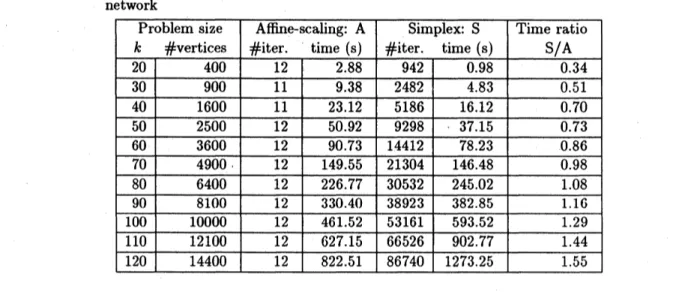
Table 3.1. Preliminary computational results for the minimum cost flow problem on $k\cross k$ grid

network

matrix multiplication by Coppersmith andWinograd [4].

When applying the interior method, a main step is to solve a linear system of equation to

compute asearch

direction

suchas the Newtondirection asmentioned above. In solving the linear

system $\tilde{A}\tilde{x}=b\sim$forthe linearprogramming problem of the form

mentioned in the beginning of the

introduction, wemainly haveto solve a linear system with a$d\cross d$symmetric matrix$\tilde{A}$

defined by

$\tilde{A}=A^{T}DA$

where$D$is adiagonal matrix whose diagonal elementsarepositive. For most interior-point methods

proposedsofar, theirsearch directioncanbe computed relatively easilyifthe linearsystem for this

$\tilde{A}$

is solvable bysome efficient method.

In the case of networkflow,themain part of the matrix $A$is the incidence matrix of underlying

graph. Suppose $A$ isexactly theincidence matrix. For this $A$, the nonzero pattem of$\tilde{A}=A^{T}DA$

exactly corresponds to the nonzero pattem ofthe adjacencymatrix ofthe same graph.

Therefore, when the network isan s(n)-separable graph, the technique ofnested dissectioncan

be applied in the main step ofthe interior-point method. By elaborating thiscombination of the

interior-point methodwith restart procedure by Vaidya [30] and the nested dissection technique in

moredetail,for the planarminimumcostflowproblem,$O(n^{1.594}\vee\Gamma og\overline{n}\log(n\gamma))$time and_{$O(n\log n)$}

space [13], where $\gamma$ is the largest absolute value amongedges costs and capacities represented by

integers. Parallelresultscorresponding to this is mentionedat the end of thepreceding subsection. When$\gamma$is polynomially bounded in$n$, the sequential time complexity becomes $O(n^{I.6})$ whichis

bestamongexisting algorithunsbya factor roughly$O(n^{0.4})$

.

These resultscan begeneralized to the

minimum cost flow problem on s(n)-separable networks such

as

three-dimensional grid networks.

Also,incomputational geometry, there arise linearprogranuningproblemshavingspecial structures

(e.g., [10]) which may be used to enhance the efficiency insolving the linear system.

In concluding thissubsection, weshow results ofacomputationalexperiment ofusingthe nested

dissection technique to the minimum cost flow problem on grid networks. In this experiment, as

aninterior-point method, the affine-scalingmethod,which would be the simplest interior-method,

isused, and at each iteration the linearsystemissolved by the nested dissection technique. Table

3.1 gives the results. Also, to compare its result withe some other method, the running time of

the network simplex code, taken from a book [17], is also shown. In the simplex method, one

iterationcorresponds to one pivoting. It should be noted that, in comparingthese two methods,

simplycomparing the running times listed here is meaningless, since these two methods use different

stopping criteria and both implementationsare not best possible at all. Instead, in the table, it

with pure linear programming theory through randomization. In this section, we mention a result

by Adler and Shamir [1] which combines a randomized algorithm with an interior-point method.

This is really a nice example of combining results in computational geometry and mathematical

programming.

The algorithm is basically similar to Clarkson’s randomized algorithm [3]. Instead of simple

uniform random sampling, it uses self-adjusting weighted random sampling and tries to keep the

number ofsampled constraints smaller with respect to $d$

.

That is, instead ofmaintaining all the

violating constraints in the Clarkson’s algorithm, this algorithmincreases, for each violating

con-straint,the probability forthe constraintto be sampled inlatersteps. Bythis strategy, throughout

the algorithm, it simply samples $O(d^{2})$ constraints, not $\Gamma n$constraintsat each stage.

In the original randomized algorithm, a subproblem is solved recursivelybythe

same

randomized algorithm until the

size

of the subproblem becomes some constant. Instead, any interior-point method may be used to solve the subproblem. Since the size of this subproblem is relatively

smallerthanthewhole size (infact, thenuunberofconstraints insubproblemsintheprocessof this

algorithm is bounded by $O(d^{2})$ with $d$ variables

as

mentioned above), the randomized algorithm

maygain somemerit from this. We skip thedetails andjust mention finalresultsin [1]. Based on

the strategy mentionedabove,itcanbe shown that the linear programmingproblem is solvablein

expected time $O((nd+d^{4}L)d\log n)$

.

_{This improves much the time complexity if} $d\ll n$_, which is

quite interesting from the viewpoint of the interior-pointmethod.

This way ofcombining the interior-point method withacertain computational-geometric

tech-nique is still na’ive. Besides this algorithm, randomization would be useful in some parts of the

interior-pointmethod,andresearchalong this line, combining thecontinuousapproachanddiscrete

approach, woulddeserve muchattention.

5

Concluding Remarks

We havediscussedabout linearprogrammingfrom the standpoints of both computationalgeometry

andmathematical programming, and have explain some fruitful results obtained through combining the ideain both fields.

In the introduction, both ofdiscrete and continuous aspects of linear programming are

men-tioned. Since discrete structures are easier to handle by computers, theoretical computer science

has

so

far pursued discrete side

very

much. In recent

years,

there have been proposed many

non-linear approach to discrete optimization problems. As in linear programming, handing nonlinear

phenomena in the theory ofdiscrete algorithms and complexity will be required in future. Even

in the lowdimensional space treatedin computational geometry, we have not yet fully understood

how to treat the

continuous

world in a

discrete

setting, and this type of

new

problems will deserve further investigation.

References

[1] I. Adler and R. Shamir: A Randomization Scheme for Speeding Up Algorithms for Linear

Programming Problems with High Constraints-to-Variables

Ratio.

DIMA CS Technical Report

89-7, DIMACS, 1989.

[2] M. Blum, R. W. Floyd, V. Pratt, R. L. Rivest andR. E. Tarjan: Time Bounds for Selection.

Joumal

_of

Computer andSystem Sciences, Vol.7 (1973), pp.448-461.

[3] K. L. Clarkson: A Las Vegas Algorithm for Linear Programming when the Dimension is Small.

Proceedings

_of

the 29th IEEE Annual Symposium on Foundations

_of

Computer Science, 1988,

pp.452-456.

[4] D.Coppersmith andS.Winograd: MatrixMultiplicationvia Arithunetic Progressions. Journal

of

Symbolic Computation, Vol.9, No.3 (1990), pp.251-280.

[5] G. Dantzig: Linear Programming and Extensions. Princeton University Press,

1963.

[6] M.

R.

Garey and D. S. Johnson: Computers and Intractability: A Guide to the Theory

_of

NP-Completeness. W. H. Freeman, San Francisco, 1979.

[7] A. George: NestedDissection ofa RegularFinite Element Mesh. SIAMJournal on Numerical

Analysis,Vol.10, No.2 (1973),

pp.345-363.

[8] A. V. Goldberg,S. A. Plotkin,D. B.Shmoys and

\’E.

Tardos: Interior-Point Methods in Parallel

Computation. Proceedings

_of

the 30th AnnualIEEE Symposium on Foundations

_of

Computer Science, 1989,

pp.350-355.

[9] D. Haussler and E. Welzel: Epsilon-Nets and Simplex Range Queries. Proceesings

_of

the 2nd

AnnualACMSymposium on Computational Geometry, 1986, pp.61-71.

[10] H. Imai: A Geometric Fitting Problem of Two Corresponding Sets of Points on a Line.

IE-ICE Transactions on Fundamentals

_of

Electronics, Communications and Computer Sciences,

Vol.E74, No.4 (1991), pp.665-668.

[11] H. Imai: On the Polynomiality of the Multiplicative Penalty

Function

Method for Linear Programmingand Related Inscribed Ellipsoids. IEICE Transactions on Fundamentals

_of

Elec-tronics, Communications and ComputerSciences, Vol.E74, No.4 (1991), pp.669-671.

[12] H. Imai, K. Kato and P. Yamamoto: A Linear-Time Algorithmfor Linear $L_{1}$ Approximation

of Points. Algorithmica, Vol.4, No.1 (1989), pp.77-96.

[13] H. Imai and K. Iwano: Efficient Sequential and Parallel Algorithms for Planar Minium

Cost

Flow.Proceedings

_of

theSIGAL International Symposium onAlgorithms(T.Asano,T.Ibaraki,

H. Imai, T. Nishizeki, eds.), Lecture Notes in Computer Science, Vol.450, Springer-Verlag,

Heidelberg, 1990, pp.21-30.

[14] M. Iri: A Proof of the Polynomiality of the Iri-Imai Method. Manuscript, to be presented at

the 14th International Symposiuun on Mathematical Programning, 1991.

[15] M. Iri and H. Imai: A Multiplicative Barrier Function Method for Linear Programming.

Al-gorithmica, Vol.1 (1986), pp.455-482.

[16] N. Karmarkar: A New Polynomial-Time Algorithm for Linear Programming. Combinatorica,

Vol.4 (1984), pp.373-395.

[17] J. L. Kennington and R. V. Helgason: Algorithms

_for

Network Programming. John Wiley

&

Apphed Mathematics, Vol.36,No.2 (1979), pp.177-189.

[22] N. Megiddo: Linear Programming in Linear Time when the Dimension is Fixed. Journal

_of

the Association

_for

Computing Machinery, Vol.31 (1984), pp.114-127.

[23] R. C. Monteiro and I. Adler: Interior Path FollowingPrimal-Dual Algorithms Part II: Convex

Quadratic Programming. Mathematical Programming, Vo..44 (1989), pp.43-66.

[24] K. Numata and T. Tokuyama: Splitting a Configuration in a Simplex. Proceedings

_of

the

SIGAL InternationalSymposium on $Algo\sqrt thms$ (T. Asano, T. Ibaraki, H. Imai, T. Nishizeki,

eds.), LectureNotesin Computer Science,Vol.450,Springer-Verlag, Heidelberg, 1990,

pp.429-438.

[25] J. B. Orlin: A Faster Strongly Polynomial Minimum Cost FlowAlgorithm. Proceedings

_of

the

20th Annual ACM Symposium on Theory

_of

Computing, 1988, pp.377-387.

[26] V. Pan and J. Reif: Efficient Parallel Solution of Linear Systems. Proceedings

_of

the 17th AnnualACM Symposium on Theory

of

$Compui\{ng$_{, Providence, 1985, pp.143-152.}

[27] F. Preparataand M. I. Shamos: Computational Geometry: An Introduction. Springer-Verlag,

New York,

1985.

[28] J. Renegar: A Polynomial-Time Algorithm, based on Newton’s Method, for Linear

Program-ming. Mathematical Programming, Vol.40 (1988), pp.59-93.

[29] T. Tokuyamaand J. Nakano: GeometricAlgorithuns for aMinimum CostAssigmnent Problem.

Proceedings

_of

the 7th AnnualACM Symposium on Computational Geometry, 1991,

pp.262-271.

[30] P. Vaidya: Speeding-Up Linear Programming Using Fast MatrixMultiplication. Proceeding

_of

the 30th AnnualIEEE Symposium on Foundations

_of

Computer Science, 1989, pp.332-337.

[31] V. N. Vapnikand A. Ya.Chervon\’enkis: On the Uniforn Convergence of Relative Frequencies of Eventsto Their Probabilities. Theory

_of

Probability and Its Applications,Vol.16, No.2 (1971), pp.264-280.

[32] S. Zhang and M. Shi:

On

Polynomial Property of Iri-Imai’s New AlgoritIun for Linear