AHP
による区間ウェイト制約を導入した
DEA
円谷
友英
,
市橋
秀友
,
田中
英夫
大阪府立大学大学院
工学研究 f:f
〒
599-8531
堺市学園町
1-1
Phone 0722-54-9355, Fax
0722-54-9915
$\mathrm{e}$
{entanl,
ichl
$1^{(\underline{\mathrm{i}\mathrm{i})}}\mathrm{i}\mathrm{e}.\mathrm{o}\mathrm{S}\mathrm{a}\mathrm{k}\mathrm{a}\mathrm{r}\mathrm{u}-\iota\iota$.acjp
1
豊橋創造大学
経営情報学部
〒
440-8511
豊橋市牛川町松下 20-1
Phone 0532-54-2111, Fax
$0.532-5\overline{:)}- 080:$
}
$\mathrm{e}$
{,
$\mathrm{a}11\mathrm{a}\mathrm{k}\mathrm{a}11^{(}\underline{\mathrm{C})}\mathrm{S}\mathrm{o}\mathrm{z}\sim_{\iota 0}$
. ac.jp
Abstract:
AHP is proposed to
give
$\mathrm{t}1_{1}\mathrm{e}$importance grade with
respect to
lIlany
items.
However,
a de
$(’ \mathrm{i}\mathrm{s}\mathrm{i}\mathrm{o}\mathrm{l}\mathrm{l}$
maker tends
to
give
the
inconsistent,
information about tlle importance
$\mathrm{g}\mathrm{r}_{\dot{\mathrm{c}}}\iota \mathrm{d}\epsilon$of input alld
outpu
$\mathrm{t}$
itelns. Then a
comparison matrix
$\mathrm{o}\mathrm{b}\mathrm{t}$,ained
by
a decision lnaker
$11_{\dot{\mathrm{t}}}1\mathrm{S}\mathrm{i}\iota \mathrm{l}\mathrm{C}\mathrm{O}\mathrm{l}\iota \mathrm{s}\mathrm{i}:’\mathrm{t}\mathrm{e}\mathrm{l}\iota \mathrm{t}\mathrm{e}\mathrm{I}\mathrm{e}\mathrm{l}\mathrm{l}\mathrm{l}\mathrm{e}\mathrm{l}\mathrm{l}\mathrm{f}\backslash .,$.
Therefore
to
deal with a decision maker’s inconsistency, interval
AHP,
where the
$\mathrm{i}_{\ln_{\mathrm{P}}}\mathrm{o}\mathrm{r}\mathrm{t}\mathrm{a}\mathrm{n}\mathrm{C}\mathrm{e}$grade of tlle item is
given
$\dot{\mathrm{c}}1S^{\neg}$an
interval,
is
proposed. Ill this paper we also
assume
$\mathrm{t}1_{1}\mathrm{a}\mathrm{t}$
a
decision
lnaker’s
$\mathrm{i}_{11\mathrm{c}\mathrm{o}}11\mathrm{s}\mathrm{i}_{\mathrm{i}},\mathrm{t}\mathrm{e}11\mathrm{c}\mathrm{v}\vee$is
represented
as an interval.
lts
center
is
obtained by
eigenvector
method and
its
radius is obtained
by
$\mathrm{i}\mathrm{l}\mathrm{l}\mathrm{t}‘ \mathrm{e}\mathrm{r}\mathrm{v}\mathrm{a}\mathrm{l}$regressioll analysis
$\mathrm{u}\mathrm{s}\mathrm{i}\mathrm{l}$
the
obtained
centers.
To clloose the crisp
$\mathrm{i}1\eta \mathrm{p}_{\mathrm{o}\mathrm{r}\mathrm{t}}\mathrm{c}\mathrm{a}\mathrm{n}\mathrm{C}\mathrm{e}$grades and
$\mathrm{t},1_{1}\mathrm{e}$
crisp efficinency
in
the
decision maker’s jtJdgelnent, we
use
DEA,
$\mathrm{w}\mathrm{h}\mathrm{i}\mathrm{C}[_{1}\mathrm{i}:’\dot{\mathrm{c}}\mathrm{t}\mathrm{l}\mathrm{l}$
evaluation
method
from
$\mathrm{t}1_{1}\mathrm{e}$optimistic viewpoint
wit,
$1_{1}$respect
to
many input, and
output
items.
The weight in DEA and
tlle
ilnportance
grade t,hrough AHP are silnilar aiid we normalize data in order
to
make tlle weight in
DEA itself represent the importance grade
in
AHP.
$\mathrm{k}\mathrm{e}.\mathrm{v}\mathrm{W}\mathrm{o}\mathrm{r}\mathrm{d}_{\mathrm{S}}:\mathrm{D}\mathrm{E}\mathrm{A}$
, AHP,
Interval importance grades
1
Introduction
The
efficiency
is
considered
as
the
ratio
of
weighted
sum of
$\mathrm{o}\mathrm{u}\mathrm{t}_{\mathrm{p}\mathrm{u}}\mathrm{t}$data to
that of input data. It
is
nat-ural to take the
$\mathrm{i}_{\ln_{\mathrm{P}^{\mathrm{O}}}}\mathrm{r}\mathrm{t}\mathrm{a}\mathrm{n}\mathrm{c}\mathrm{e}$grade
of an
item
$\mathrm{a}^{\neg}$its weight,.
However,
it is
not,
usually
easy for a
decision maker to give the determined importance
grade directly. Therefore, AHP
(Allalytic
Hierar-chical
Process)
is
proposed to determine the
im-portance
grades of eacb
item
[1].
AHP
is
a method
to
deal
$\backslash \mathrm{v}\mathrm{i}\mathrm{t}\mathrm{l}\mathrm{l}$the
$\mathrm{i}_{111}\mathrm{p}\mathrm{o}\mathrm{r}\mathrm{t}\mathrm{a}11\mathrm{C}\mathrm{e}$
grarles witll respect
to
lnany
items.
In
conventional
AHP,
the crisp
importance grade of
$\mathrm{e}\mathrm{a}\mathrm{c}1_{1}\mathrm{i}\mathrm{t}\mathrm{e}\ln$can be obtained
by
solving
eigenvector
problem
witll
a
compari-son nlatrix
$\mathrm{W}1_{1\mathrm{o}\mathrm{s}\mathrm{e}}$elements are
given
by a
decision
$111_{\mathrm{C}}^{\prime\iota \mathrm{k}}\mathrm{e}\mathrm{r}$
by
$\mathrm{C}\mathrm{o}\mathrm{m}\mathrm{p}\mathrm{a}\mathrm{r}\mathrm{i}_{1\mathrm{l}}\mathrm{g}$
all possible
pairs
of
items.
Based on
$\mathrm{t}_{\mathrm{c}}\mathrm{h}\mathrm{e}$idea that a
$1_{1\mathrm{U}1}\mathrm{n}\mathrm{a}\mathrm{n}$judgement
is
in-collsistent,
the estimated weights should
contains
uncertainty.
Tbus,
the model tbat
gives the
im-portance
grade
c1S
an
int,erval
to
reflect
t,he
incon-sisCellcy of a comparison
matrix is
proposed [2].
We
take another way to obtain the interval
im-portallce
grades based on
eigenvector method and
illterval
regression
analysis.
Assuming
that the
es-$\mathrm{t}\mathrm{i}_{1}\mathrm{n}\mathrm{a}\mathrm{t}\mathrm{e}\mathrm{d}$
weight is an
$\mathrm{i}_{11}\mathrm{t}\mathrm{e}\mathrm{r}\mathrm{v}\mathrm{a}1$denoted by
its center
alld
its
raclius, two
problems
for
finding the
cen-ter
alld the
radius are formulated.
$\mathrm{T}1_{1}\mathrm{e}$centers are
$\mathrm{o}\mathrm{b}\mathrm{f}$
,ained
by
eigenvector
method
in
the
salne
way
as
$\mathrm{C}\mathrm{o}11\mathrm{v}\mathrm{e}\mathrm{l}\mathrm{l}\mathrm{t}_{1}\mathrm{i}\mathrm{o}11\mathrm{a}1$AI-IP.
Usillg
$\mathrm{t}1_{1}\mathrm{e}$obt,ained
cellters,
the radius
is
obtained
$\mathrm{b}_{*}\mathrm{v}$interval
regression
anal-ysis where each radius
is
minimized subject
to
tbe
const,raint
collditions
$\mathrm{t}1_{1}\mathrm{a}\mathrm{t}$t,he
estimated
intervals
include the elements of the given
$\mathrm{c}\mathrm{o}\mathrm{l}\mathrm{n}\mathrm{p}\mathrm{a}\mathrm{r}\mathrm{i}_{\mathrm{S}\mathrm{o}}11$ma-tlix [3]. Wllen a decision lllaker
gives
comparison
matrices
for input alld
$\mathrm{o}\mathrm{t}\mathrm{l}\mathrm{t}_{\mathrm{P}^{\iota 1\mathrm{t}}}$items,
the
$\mathrm{i}_{11}\mathrm{t}\mathrm{e}\mathrm{r}-$val importance grades of input and output items
are obtained respectively. The obtailled interval
importance
grades
can be considered as the
ac-ceptable
$\mathrm{i}\mathrm{n}1\mathrm{p}_{0}\mathrm{r}\mathrm{t}\mathrm{a}11\mathrm{c}\mathrm{e}$grades for a decision lnaker.
To
give
tbe crisp efficiency, we clloose the
$\mathrm{n}\mathrm{l}\mathrm{o}\mathrm{s}\mathrm{t}$optimistic importance grades
lor
the analyzed
ob-ject in the interval
by
DEA
(Dat,a
$\mathrm{E}11\mathrm{e}\mathrm{l}\mathrm{o}_{\mathrm{P}^{1}}11\mathrm{e}11\mathrm{t}$Allalysis)
$[4][,5]$
. DEA is
a
well-known method
to
evaluate
DMUs
(
$\mathrm{D}\mathrm{e}\mathrm{c}\mathrm{i}\mathrm{S}\mathrm{i}\mathrm{o}\mathrm{l}\mathrm{l}\mathrm{M}\mathrm{a}\mathrm{k}\mathrm{i}_{1\mathrm{l}}\mathrm{g}$Units)
$\mathrm{f}\mathrm{r}\mathrm{o}\ln \mathrm{t}[_{1\mathrm{e}}$ $\mathrm{o}\mathrm{p}\mathrm{t}\mathrm{i}_{1\Pi}\mathrm{i}\mathrm{S}\mathrm{t}\mathrm{i}_{\mathrm{C}}$viewpoint. The weights in DEA and
the
import,ance
gr\v{c}tdes t,llrough
AHP
are silnilar
then DEA
is
used
to
choose the most optimistic
inuportance grades of input and output itelns
in
the decision maker’s acceptable
ranges.
In
order
to make
the weight
in
DEA
represellt
the
$\mathrm{i}_{\ln_{\mathrm{P}^{\mathrm{o}\mathrm{r}}}}-$tance
grade through AHP
itself,
we llormalize all
data
based on
$DM[\gamma_{\mathrm{o}}$
.
The
efficiencies obtained
from
tlle normalized data and tlle original data are
equal.
$\mathrm{T}1_{1}\mathrm{e}$study
$\mathrm{w}\mathrm{i}\mathrm{t}_{\iota}$]
$1$
respect
to
$\mathrm{c}\mathrm{o}\mathrm{l}\mathrm{n}\mathrm{b}\mathrm{i}_{11\mathrm{a}\uparrow},\mathrm{i}_{0}11$of
AHP and DEA was done
in
[6], where the interval
importance grades are obtained througb interval
AHP
wit,
$1_{1}$an
illter
${ }$$‘\iota 1\mathrm{c}\mathrm{o}111\mathrm{P}^{\mathrm{a}\mathrm{r}\mathrm{i}}.\aleph- \mathrm{O}11$mat,rix
and tlley
Our
proposed
$\mathrm{c}\mathrm{t}\prime \mathrm{p}\mathrm{p}\mathrm{r}oi\iota \mathrm{t}\mathrm{l}\mathrm{l}\mathrm{e}\mathrm{s}$to
obtaill
t,he
inter-val
$\mathrm{i}\mathrm{r}\mathrm{n}\mathrm{p}\mathrm{o}\mathrm{r}\mathrm{f}\mathrm{a}\mathrm{n}\mathrm{c}\mathrm{e}$grades and
to
$\mathrm{i}\mathrm{t}\mathrm{l}\mathrm{t}_{c}\mathrm{r}\mathrm{o}\mathrm{d}11\mathrm{C}\mathrm{e}\mathrm{t},1\iota \mathrm{e}\ln$t,o
DEA
are
$\mathrm{d}\mathrm{i}\mathrm{I}\mathrm{r}\mathrm{e}\Gamma \mathrm{e}\mathrm{l}\mathrm{l}\mathrm{t}\mathrm{f}\mathrm{r}\mathrm{o}\mathrm{n}1\mathrm{t},1_{1}\mathrm{e}$study [6]
$\mathrm{i}1\iota \mathrm{t}‘|\mathrm{l}\mathrm{e}$sellse
of
$\mathrm{t}1_{1\dot{\mathrm{c}}1}1,$
otll
$\dot{(}\iota \mathrm{i}111$is
to
clloose
$\mathrm{t}_{0}11\mathrm{e}$import,ance grades
ill a possible
ranges
$\mathrm{w}11\mathrm{i}\mathrm{c}1_{1}$are
$\mathrm{e}\mathrm{s}\mathrm{t}\mathrm{i}_{1\eta}\mathrm{a}\mathrm{t}‘ \mathrm{e}\mathrm{d}$from a
decision maker’s judgement.
2
Interval AHP
When
$\mathrm{t}1_{1}\mathrm{e}\mathrm{r}\mathrm{e}$are
$?l$
items
$I_{1},$
$\ldots,$
$I_{\iota},$
,
a
decision
maker
$\mathrm{c}\mathrm{o}\mathrm{n}\mathrm{l}\mathrm{p}\mathrm{a}\mathrm{r}\infty$a pair of
items
for all possible pairs
tllell
we can obtain a comparison
matrix
$A$
as follows.
$.-[=(o_{n1}a\cdot..\cdot$
)
$1\sim 1$ $a_{1\underline{)},1}..\cdot.\cdot\cdot$.
$.\cdot...\cdot.\cdot.\cdot.\cdot$ $\mathit{0}\cdot...$)
$a_{1n}\sim 1r\iota)$
$\mathrm{W}[_{1\mathrm{e}\mathrm{r}\mathrm{e}}\mathrm{t}1_{1}\mathrm{e}$
element of
matrix
$A,$
$\mathit{0}_{ij}$
,
shows the
im-portallce
grade of
$I_{i}$obtained by
comparing
with
$I_{j}$
,
the orthogonal elements
are
equal to 1, that
is
$c/_{ii}=1$
and the reciprocal property
is
satisfied,
tllat
is
$\mathit{0}_{ij}=1/a_{ji}$
.
The
more the number of
compared
items
be-come,
the
more difficult
it is
to
give consistent
comparison
values,
since
a
decision nuaker
com-pare only two
items
at
one
time.
The obtained
colnparison
matrix
has
inconsistent
elements each
other.
$\mathrm{T}1_{1\mathrm{e}\Gamma \mathrm{e}}\mathrm{f}\mathrm{o}\mathrm{r}\mathrm{e}$,
it is
more
suitable to
give
$\mathrm{t}1_{1}\mathrm{e}$items interval importance grades and partial
or-der of
t,he
items is
obtained by them.
Then,
we
estimate
the ilnportance
grade
of
item
$i$
,
as an
in-t,erval
denoted
as
$[_{J}V_{i}$,
that
is determined by
its
center
$\mathrm{u})^{C}i$and
its
radius
$d_{i}$as
follows.
$\nu V_{i}=[^{\iota_{1},\iota C}\iota_{i,i}r1A)]=[\iota\iota’ i-di, \mathfrak{l}\iota_{i})+d_{i}C]$
$\backslash \mathrm{v}\iota \mathrm{l}\mathrm{e}\mathrm{r}\mathrm{e}L_{\mathrm{l}v_{i}}$
and
$U_{mi}$
are
the
$\mathrm{u}_{\mathrm{P}1^{\mathrm{J}\mathrm{e}\mathrm{r}}}$and the
lower
$|)0\iota 11\iota \mathrm{d}.\backslash$
or
the illterval. In order
to
deterlnine
in-terval import,
$\mathrm{a}\mathrm{l}\iota \mathrm{c}\mathrm{e}$grades, we have
two
problenis
where
olle
is
to
obtain the
center
and
the
ot,ller
is
to
obtain the
radius. The center is obtained by
eigenvector
llletllod with the obtained
comparison
$11\mathrm{u}\mathrm{a}\mathrm{t}\Gamma \mathrm{i}_{\mathrm{X}}A$.
The
eigenvector problem
is
formulated
as follows.
$Aw=\lambda w$
(1)
$\mathrm{w}1_{1\mathrm{e}}\mathrm{r}\mathrm{e}\lambda$
is
$\mathrm{t}\mathrm{l}\mathrm{l}\mathrm{e}$eigenvalue,
$w$
is
the
eigenvector
and
tlley
are the decision variables of this probelm.
$\mathrm{S}\mathrm{o}\mathrm{l}\mathrm{V}\mathrm{i}\mathrm{l}\iota \mathrm{g}(1),$
tlle
$\mathrm{e}\mathrm{i}\mathrm{g}\mathrm{e}\iota \mathrm{l}\mathrm{v}\mathrm{e}\mathrm{C}\mathrm{t}\mathrm{o}\mathrm{r}(w_{1}^{c}, \ldots , \iota v_{n}^{c})$for
the
principal
eigenvalue
$\lambda_{t’ 1ax}$
is
obtained as the
cen-ter
of the illterval
$\mathrm{i}\ln$[
$)\mathrm{o}\mathrm{r}\tan_{C}\mathrm{C}\mathrm{e}.\mathrm{g}\mathrm{r}*\mathrm{a}\mathrm{d}\mathrm{e}\mathrm{s}$of
each
it,enl
$(I_{1}, \ldots , I_{f1})$
.
The center
$n_{i}$
’
$1\mathrm{S}$normalized to be
$\sum^{\prime \mathrm{i}}i=\iota^{\mathrm{t}}1‘ ic*=1$
.
The
$\mathrm{r}\mathrm{a}\mathrm{d}\mathrm{i}\mathrm{l}\mathrm{l}‘\backslash$is
obtained
based
on
$\mathrm{i}_{11\mathrm{t}\mathrm{a}}\mathrm{e}\mathrm{r}1$re-gression
analysis,
which
is
to
$\mathrm{f}\mathrm{i}_{11}\mathrm{d}$the estimated
$\mathrm{i}_{11}1_{}(3\mathrm{r}\mathrm{v}_{\dot{\mathrm{c}}1}1\backslash .,$
to
$\mathrm{i}_{1\iota(}\cdot||1\mathrm{t}[\mathrm{e}\mathrm{t}[\mathrm{l}\mathrm{e}\mathrm{o}\mathrm{l}\mathrm{i}\mathrm{g}\mathrm{i}\iota 1i||$
dat,a.
$111$
our
prob-lem,
($/ij$
is
$\dot{(}|\mathrm{p}\mathrm{p}\mathrm{r}\mathrm{o}\mathrm{X}\mathrm{i}_{11}1\mathrm{a}\mathrm{t}\mathrm{G}\mathrm{d}_{\dot{\subset}}1\mathrm{S}’‘\iota \mathrm{t}|\mathrm{i}_{11}\downarrow \mathrm{e}\mathrm{r}\mathrm{V}\dot{\mathrm{t}}\iota \mathrm{I}$ratio i’llcll
that
the
$\iota_{0}||0\backslash \mathrm{V}\mathrm{i}_{1}\mathrm{r}\mathrm{e}\mathrm{l}\mathrm{a}\mathrm{t}(\mathrm{i}\mathrm{o}\mathrm{l}\mathrm{l}$holds.
$o_{\mathrm{i}j} \in\frac{||’}{11’}\perp=\mathrm{j}[\frac{1v^{\mathrm{c}}-d_{1}}{\mathrm{t}\mathrm{t}_{g}^{1}+\mathrm{c}\cdot d_{\mathrm{j}}}.,$ $\frac{\mathrm{c}v^{\mathrm{c}}+(l\prime}{1v_{j}^{c}-l_{\mathrm{J}}}.\cdot‘]$
(2)
where
$\mathfrak{s}\prime V_{i}^{\vee}(\mathrm{t}\prime 11\mathfrak{c}1\dagger l_{j}^{\mathit{1}}’$arc
$\mathrm{t}1_{1}\mathrm{e}(^{1}.\backslash \mathrm{t}\mathrm{i}_{\ln}\mathrm{a}\mathrm{t}\mathrm{e}\mathrm{d}$inteval
impor-tance
$\mathrm{g}\mathrm{r}_{\epsilon\backslash }\mathrm{d}\mathrm{e}\mathrm{s}\backslash \mathrm{a}1\iota \mathrm{d}\ovalbox{\tt\small REJECT} V_{i}/\nu V_{j}$is
defined as the
lllaxi-nlulll
range.
The
$\mathrm{i}11\mathrm{t}\mathrm{e}\mathrm{r}\mathrm{v}\dot{\mathrm{c}}\mathrm{t}[\mathrm{i}\mathrm{I}11\mathrm{p}_{\mathrm{o}\mathrm{r}}\mathrm{f},\mathrm{a}11\mathrm{c}\mathrm{e}$grades are
$\det_{\mathrm{C}\mathrm{r}111}\mathrm{i}11\mathrm{e}\mathrm{d}$in
consideration of the
$\mathrm{i}11\mathrm{c}\mathrm{o}11\mathrm{S}\mathrm{i}_{\mathrm{S}}\mathrm{t}\mathrm{e}\mathrm{n}\mathrm{c}\backslash .$’
contained
in
a colllparison matrix. With
using
tlle obtained
$\mathrm{c}\mathrm{e}\mathrm{n}\mathrm{t}\mathrm{e}\mathrm{r}\mathrm{s}n_{i}’ \mathrm{c}$
’
by (1),
the
radius should be
$\iota \mathrm{n}\mathrm{i}_{1\mathrm{l}}\mathrm{i}\mathrm{m}\mathrm{i}\mathrm{Z}\mathrm{e}\mathrm{d}$subject
to
$\downarrow 1_{1e\mathrm{C}\mathrm{o}}11\mathrm{s}\mathrm{t}1^{\cdot}\mathrm{c}l\prime \mathrm{i}_{1}1\mathrm{t}$condit
ions
$\mathrm{t}\mathrm{l}\mathrm{l}\dot{\mathrm{c}}\mathrm{t}\{\mathrm{t}\mathrm{l}\downarrow \mathrm{e}$rela-tioll
(2)
for
all
$\mathrm{e}\mathrm{l}\mathrm{e}\mathrm{l}\mathrm{l}$)
$\mathrm{e}\mathrm{l}\mathrm{l}\mathrm{t}\mathrm{S}\mathrm{s}\mathrm{l}\mathrm{l}0\mathrm{I}\mathrm{l}\downarrow \mathrm{d}$be satisfied.
nlill
$\lambda$$\mathrm{s}.\mathrm{t}$
.
$\frac{\iota v_{\mathrm{i}}^{C\vee}-d_{i}}{w_{j}^{c*}+d_{j}}\leq a_{ij}\leq\frac{w_{i}^{c*}+d_{i}}{w_{j}^{c*}-d_{j}}$
,
(.3)
$i=1,$
$\ldots,$
$n-1,$
$j=i+1,$
$\ldots,$
$n$
$d_{i}\leq\lambda$
,
$i=1,$
$\ldots,$
$n$
The
first
constraint condition shows the
in.clusion
relation
(2).
Instead of
minilnizillg the sum of
radii,
we nuillilnize the
$\mathrm{m}\mathrm{a}\mathrm{x}\mathrm{i}_{\ln}\mathrm{u}\mathrm{I}1$of them.
This
can be reduced to
LP problenl. The radius
$0[\mathrm{t}1_{1\mathrm{e}}$interval importance grades reflect
some
illconsis-tency
in
the
given
mat,
$\mathrm{r}\mathrm{i}\mathrm{x}$.
In
other words, the
obtained importance grades
can
be regarded as
the possible
ranges
estinlated from the
given
data.
The interval
$\mathrm{i}_{1}\mathrm{n}\mathrm{p}_{0}\mathrm{r}\mathrm{t}\mathrm{a}\mathrm{n}\mathrm{c}\mathrm{e}$grade shows the
accept-able
range
for
a decision maker.
3
Choice of the
$\mathrm{o}_{\mathrm{P}}\mathrm{t}\mathrm{i}\mathrm{n}\mathrm{l}\mathrm{i}_{\mathrm{S}\mathrm{t}\mathrm{i}\mathrm{c}}$$\mathrm{w}\mathrm{e}\mathrm{i}\mathrm{g}\mathrm{l}_{1}\mathrm{t}\mathrm{S}$
and efficiellcy
by DEA
3.1
DEA
with the normalized data
$\ln$
DEA tbe
$[\mathrm{n}\mathrm{a}\mathrm{x}\mathrm{i}_{1}11\mathrm{u}\mathrm{t}1]$ratio
of
$0\iota 1\mathrm{t}_{\mathrm{P}}\mathrm{U}\mathrm{t}$
data
to
input
$\mathrm{d}\mathrm{a}1_{}\mathrm{a}$is assumed as
$\mathrm{t}\mathrm{l}\iota \mathrm{e}\mathrm{e}t\mathrm{t}\mathrm{i}(\mathrm{i}\mathrm{e}\mathrm{l}\iota \mathrm{c}\mathrm{y}$alld
it is
calculated from the optimistic
$\mathrm{v}\mathrm{i}\mathrm{e}$}
$\mathrm{v}\mathrm{p}_{\mathrm{o}\mathrm{i}_{11}\mathrm{t}}$for each
DMU. The basic DEA lnodel
is
$\mathrm{f}_{\mathrm{o}\mathrm{r}}\mathrm{n}\mathrm{l}\mathrm{U}\mathrm{l}\mathrm{a}\mathrm{t}\mathrm{e}\mathrm{d}$as
fol-lowing LP problem.
$\theta_{o}^{E^{*};}=\mathrm{l}\mathrm{n}\mathrm{a}\mathrm{X}uy_{\mathit{0}}u$
$\mathrm{s}.\mathrm{t}$
.
$v^{t_{X_{o}}}$
$=1$
$-\tau’ {}^{t}X+?lYt$
$\leq 0$
(4)
$u$
$\geq 0$
$v$
$\geq 0$
where the decision variables
are the weight vectors
$u$
alld
$v,$
$X\in$
)
$)_{\mathrm{I}}^{\backslash n\}}\cross n\mathrm{a}\mathrm{l}\iota \mathrm{d}Y\in\Re^{k\mathrm{x}n}$are
$\mathrm{i}_{11}\mathrm{P}^{\mathrm{U}}\mathrm{t}$and
output
mat,rices
consisting
of all input. and
out-put
vectors
t,hat
are
all positive altd
$\mathrm{t}[\mathrm{t}\mathrm{e}$lllllnber
of
DMUs
is
$n$
.
(4)
gives
the opt,imistic
$\mathrm{t}\mathrm{v}\mathrm{e}\mathrm{i}\mathrm{g}[\mathrm{l}\mathrm{t}\mathrm{S},$$u.\mathrm{r}$them. In
case
that the opt,imal value of the
ob-$\mathrm{j}\mathrm{e}\mathrm{c}\mathrm{f}_{\downarrow}\mathrm{i}\mathrm{v}\mathrm{e}$fullctioll is
equal to 1, the optinlal
weights
are
not,
determined
identically.
In
$\mathrm{C}\mathrm{O}11\mathrm{v}\mathrm{e}11\mathrm{t},\mathrm{i}_{\mathrm{o}\mathrm{n}\mathrm{a}}1$DEA
(4),
it is
difficult
t,o
dis-cuss
tbe importance grades of input and output
items
by
comparing
t,heir
weights, because they
depend on tlle scal
es
of
$\mathrm{t}‘ 1_{1}\mathrm{e}$original
data.
The
er-ficiellcy
is
obtained as
$\mathrm{t}\mathrm{l}\mathrm{l}\mathrm{e}$ratio
of tlle hypothetical
output to
t,he
$\mathrm{h}\mathrm{y}\mathrm{p}_{\mathrm{o}\mathrm{t}_{}}1\mathrm{l}\mathrm{e}\mathrm{t}\mathrm{i}\mathrm{c}\mathrm{a}$[
input, wllere the
prod-ucts of data and weights
are
sulnlned up. It
can
be
said
that,
the product of data and
weight
rep-resents tlle
$\mathrm{i}_{1}\mathrm{n}\mathrm{p}_{0}\mathrm{r}\mathrm{t}\mathrm{a}\mathrm{n}\mathrm{c}\mathrm{e}$grade
in
evaluation
more
exact,ly
$\mathrm{t}\mathrm{l}\mathrm{l}\mathrm{a}\mathrm{n}$the
weights
only.
Then
we
llorlnalize
$\mathrm{t}1_{1}\mathrm{e}$
given
input and output data
$\mathrm{b}_{\mathrm{c}}\mathrm{o}\mathrm{e}^{\neg}\mathrm{e}\mathrm{d}$on
$DMU_{o}$
so that the input and output weights represent the
importance
grades
of
the
items.
The
normalized
input and output denoted
as
$\hat{x}_{jp}$
and
$\hat{y}_{jr}$,
$(j=1, \ldots , n)$
are obtained as follows.
$\hat{x}_{jp}$$=x_{jp}/x_{op}$
,
$p=1,$
$\ldots,$
$m$
$\hat{y}_{j},$
.
$=y_{jr}/y_{\mathit{0}},.$
,
$’$.
$=1,$
$\ldots,$
$h$
The
problem to obtain the efficiency with
the
normalized input and
output
are forlllulated as
follows.
$\theta_{o}^{E}$
.
$=$
$\max u^{t}\hat{\tau}/_{\mathit{0}}$
.
$\mathrm{s}.\mathrm{t}.\cdot=$$v^{t}\overline{x}_{o}=u1$
$-v^{r_{\hat{\mathrm{Y}}},t}+u\hat{Y}\leq 0$
${ }$.
(5)
.:
..
$.u\geq 0$
$..\prime r$.
$v\geq 0$
$\backslash \mathrm{v}1_{1\mathrm{e}\mathrm{r}}\mathrm{e}J\hat{\mathrm{Y}}$,
$\hat{Y}\mathrm{a}\mathrm{l}\mathrm{e}$the all normalized data alld
de-noted as
follows.
1
$\mathit{0}$$n$
$\mathrm{z}\grave{\mathrm{Y}}$
.
$=$
$\hat{Y}=$
The efficiellcy
fronl
$\mathrm{t}\mathrm{l}\mathrm{l}\mathrm{e}$normalized input and
output is equal
to
that fronl the origillal data by
conventional DEA. This
fact
can be verified
by
simple
calculation.
$\mathrm{A}_{\mathrm{S}\mathrm{S}\mathrm{U}}111\mathrm{i}\mathrm{n}\mathrm{g}\mathrm{t},1_{1}\mathrm{e}$
optimal solutions of
(5)
as
$u^{*}=$
$(u_{1^{*}}, \ldots , u\kappa^{*}.)^{t}$
and
$v^{*}=(v_{1^{*}}, \ldots, v_{m^{*}})^{t}$
,
tlle
following relation
can
be easily
found.
$\theta_{o}^{E}\mathrm{r}=u_{1^{*}}+\cdots+u_{\mathrm{t}^{*}}$
.
$v_{1^{*}}.+\cdots+v,|1^{*}=1$
The
above two equatiolls
follow
t,hat
the
ob-tained weight
represents tlle import,allce
grade
it-self. Then we can
use
DEA with tlle
normalized
data
t,o
choose
tlle
$\mathrm{o}\mathrm{p}\mathrm{t}\mathrm{i}_{11}1\mathrm{i}\mathrm{s}\mathrm{t}\mathrm{i}\mathrm{c}\mathrm{w}\mathrm{e}\mathrm{i}\mathrm{g}\mathrm{l}_{1}\mathrm{t}$,
in the
ill-t.erval ilnportallce grade obtained
by a
decision
lnaker
$\mathrm{t}_{:}1_{1\mathrm{r}\mathrm{o}\mathrm{u}}\mathrm{g}$]
$1\mathrm{i}_{11\mathrm{t}\mathrm{V}\mathrm{a}}\mathrm{e}\mathrm{r}1$AHP.
3.2
Optimistic importance grades in
interval importance grades
$\mathrm{T}[_{1\mathrm{e}}\mathrm{i}_{\mathrm{I}}11$
[
$)0\iota\cdot \mathrm{t}‘ \mathrm{a}|1\mathrm{C}\mathrm{e}$grades
or
output
(
$|\mathrm{t}\mathrm{l}\mathrm{C}$[
$\mathrm{i}_{\mathrm{l}1}\mathrm{p}\iota 1\mathrm{t}$iteltls
obt,ained
by
$\mathrm{c}\mathrm{o}\mathrm{t}\mathrm{l}\mathrm{l}$[
$)\mathrm{a}\mathrm{r}\mathrm{i}.\mathrm{b}\mathrm{O}\mathrm{I}\mathrm{l}11\mathrm{t}_{\dot{(}}\iota \mathrm{f}1^{\cdot}\mathrm{i}\mathrm{c}\mathrm{e}.9$
$\mathrm{g}\mathrm{i}\mathrm{V}\mathrm{e}\mathrm{l}\mathrm{l}$$1_{\mathrm{J}}\mathrm{y}$
a
$\mathrm{c}\mathrm{l}\mathrm{e}(:\mathrm{i}-$sion
maker are calculated as
$\downarrow_{j}11\mathrm{e}$following
$\mathrm{i}\mathrm{l}\mathrm{l}\mathrm{t}\mathrm{e}\mathrm{l}\cdot\mathrm{a}\mathrm{l}\mathrm{s}$through
int,erval
AHP.
$|/V_{p\rho}^{il}’=[Li|1, uin]\mathrm{t}\iota’\iota v_{\mathcal{P}},$
$p=1,$
$\cdots,$
$?’ 1$
$\nu V_{r}^{ou\iota}=[^{Lu1U}\iota v_{r}o,w^{\mathit{0}u}]\prime t,$
$\uparrow$.
$=1,$
$\cdots,$
$k$
The
centels
or
the
interval importance grades
of input and output
items
tllrougll AHP
sunl
up
to
one.
On
the
$0\dagger$,her
hand
$\mathrm{i}1\downarrow$DEA with the
nor-malized
$\mathrm{d}\mathrm{a}\mathrm{t},\mathrm{a}$,
input and
output
weights
$\mathrm{s}\mathrm{u}\ln$
up
to
one and the efficiency respectively. We obtain the
optimistic weights and efficiency through DEA by
considering the interval importance grades through
interval AHP
as
the
$\mathrm{w}\mathrm{e}\mathrm{i}\mathrm{g}\mathrm{l}_{1}\mathrm{t}$constraints in
DEA.
By
DEA,
we
can determine the
optimistic
weigllts
for
eachc
DMU in
the possible
ranges.
The input,
weights
are constrained
by
the
$\mathrm{o}\mathrm{b}\mathrm{t}$,ained
interval
importance
grades
directly
and
we
need
to
mod-ify
the
output
weights so
tllat the
sum
of them
should be
one because the obtained
importance
grades sum up
to
one.
The
constraint
conditions
for
t,he
input
and output
weights are as
$\mathrm{f}o$]
$[\mathit{0}\backslash \mathrm{s}$.
$L_{w_{p}^{in}}L_{w_{r}}out \leq\frac{\mathrm{r}/}{\sum_{p}^{k}\leq^{b_{w}^{u}}r=r}\leq U\leq vinw|\mathit{0}.ut$
,
$\uparrow$.
$=1,$
$\cdots,$
$k$
(6)
$\mathrm{p}$
,
$p=1,$
$\cdots,$
$m$
where
$u_{r}$
alld
$v_{p}$
are
$\mathrm{t}1_{1}\mathrm{e}$
variables
in
DEA alld
$L_{\mathrm{t}v_{r}^{ou\iota}},$
$U_{w_{r}^{out}},$
$L_{\iota v_{\mathrm{P}}^{i\prime}}1$and
$U_{u^{in},},$
,
are tbe bounds of
tlle
interval importance
$\mathrm{g}\mathrm{r}\prime \mathrm{d}$des of input
$p$
and
out-put
$r$
.
$\mathrm{T}1\mathrm{l}\mathrm{e}$problem to choose tlle
most
opt,imistic
weights for
$D\Lambda fU_{o}$
in
a decision maker’s
judge-mellt
is forlnulated as
follows by adding
(6)
to
(5)
as
the
constraint
conditiolls.
$\theta_{o}^{E^{*}}$
$= \max\sum_{r=1}^{k}u_{r}$
$\mathrm{s}.\mathrm{t}$.
$\sum_{\rho=1p}^{m}uv=1$
$-v^{\iota_{d}}\hat{\backslash }’+u\ddot{Y}t<0$
$u_{r}u,$.
$\leq\geq L_{lL^{1}r_{\mathit{0}}}o.uttu’$
,
$\uparrow\cdot.=1?=1’,$
$\cdot.\cdot.\cdot.’,$$kh$
.
$\langle$7)
$v_{\rho}\geq^{L}w_{\rho}^{in},$
$p=1,$
$\ldots,$
$m$
$v_{l)}\leq^{U}w_{p}^{in},$
$p=1,$
$\ldots,$
$??1$
$u\geq 0$
By data
normalization,
the
interval importance
grades
are
used
as tlle weigllt
const,raints
natu-rally, because the weight itself represents the
im-$\mathrm{P}\mathrm{o}\mathrm{r}\mathrm{t}\mathrm{a}\mathrm{n}\mathrm{c}\mathrm{e}$
grade.
In
case
$\mathrm{t}\mathrm{l}\mathrm{l}\mathrm{a}\mathrm{t}$
the efficiency
is
equal
to
one,
$\mathrm{t}_{}11\mathrm{e}$weigbts are
llot,
deternlilled identieally,
even
thollgll
all.v
weights
$\mathrm{t}\mathrm{l}\mathrm{l}\mathrm{l}\mathrm{a}\uparrow$give
the
efficiency
4
$\mathrm{N}\mathrm{u}\mathrm{n}\mathrm{l}\mathrm{e}\Gamma \mathrm{i}\mathrm{c}\mathrm{l}$example
We use one
$\mathrm{i}_{\mathrm{l}1}\mathrm{p}\mathrm{u}\mathrm{t}$and four output,
$\mathrm{s}$dat,a
shown
in
Table
1
$\mathrm{c}\mathrm{t}\prime s$all
$\mathrm{e}\mathrm{x}\mathrm{a}\mathrm{n}\tau \mathrm{P}\mathrm{l}\mathrm{e}\mathrm{w}1_{1}\mathrm{e}\mathrm{r}\mathrm{e}$A,...,J
are
denot,ed
as DMUs.
Table
1:
Data with 1-input and 4-output
The
comparison nlatrix
given
by
a decision
maker is shown
in
Table
2.
By
$\mathrm{t}\mathrm{l}\mathrm{l}\mathrm{e}\mathrm{e}\mathrm{i}\mathrm{g}\mathrm{e}\mathrm{l}\mathrm{l}\mathrm{e}\mathrm{c}\mathrm{t}\mathrm{o}\mathrm{r}$problelll
(1),
the centers of the
$\mathrm{i}\mathrm{n}\mathrm{l}\mathrm{p}\mathrm{o}\mathrm{r}\mathrm{t}\mathrm{a}\mathrm{n}\mathrm{c}\mathrm{e}$grades
of output
itenns
are obtained
as
follows.
$(\mathrm{t}_{1’ \mathrm{a}^{\wedge}’ 4}^{\}^{c*}w\cdot,,1}C\sim*,cC*ul)=$
(0.080, 0.583,
0.051,
0.286)
The radius
is
obtained by
(3)
and
the
interval
im-portance
grades are
also
shown
in Table 2.
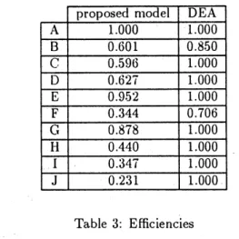
With
using
$\mathrm{t},1\mathrm{l}\mathrm{e}$llormalized
data,
$\mathrm{t}\mathrm{l}\iota \mathrm{e}$efficien-cies
obtained
by
the proposed nlodel
(7)
and by
conventional
DEA
(5)
are
$\mathrm{s}\mathrm{l}_{\mathrm{l}\mathrm{O}}\backslash \mathrm{v}11$ill Table
3.
The
efficiency
tbrough DEA
is
cletertllined only from
the
lllost
opt,imistic viewpoint for
$\mathrm{e}\dot{\mathrm{c}}\mathrm{t}\mathrm{c}\mathrm{l}\mathrm{l}$DMU
$\mathrm{w}\mathrm{i}\mathrm{C}[_{1^{-}}$out,
considering any decision lnaker’s judgement.
Ill the proposed model,
$\mathrm{t}\mathrm{l}\mathrm{l}\mathrm{e}$efficiency
can
be
ob-tained from the most
$\mathrm{o}\mathrm{p}\mathrm{t}\mathrm{i}_{1}\mathrm{n}\mathrm{i}_{\mathrm{S}\mathrm{t}\mathrm{i}\mathrm{c}}$viewpoint
for each
DMU in
a decision maker’s acceptable importance
grades.
Therefore,
the efficiencies
in
the proposed
model
are smaller
t,han
those
in conventional
DEA.
We pick out
$\mathrm{B}$alld
$\mathrm{C}$to
remark tlle result ill
view of
$\mathrm{t}1_{1}\mathrm{e}$cllosetl weights in Table 4 and
Fig-ure 1.
In
Table
4,
the
$\mathrm{c}1_{1}\mathrm{o}\mathrm{s}\mathrm{e}\mathrm{n}$output
weights
and the efficiencies
by
the proposed model are
Table
2:
Comparison
$1\mathrm{n}\mathrm{a}\mathrm{t}\mathrm{r}\mathrm{i}_{\mathrm{X}}$alld
illlportaIlce
gracles
of
t,be
output
$\mathrm{i}\mathrm{I},\mathrm{e}\mathrm{l}\mathrm{l}\mathrm{l}\mathrm{s}$Table
3:
Efficiencies
shown.
The
sums
of the
obtained weights are
normalized to
one.
All the weights show the
op-timistic
ones in the obtained interval importance
grades. In Figure 1, where the lines show the
in-terval importance grades through inin-terval
AHP
and
$\cross$and
$0$
show
$\mathrm{t}\mathrm{l}\grave{\lambda}\mathrm{e}$chosen weights that
give
the
efficiencies
of
$\mathrm{B}$and
$\mathrm{C}$respectively.
The
de-cision
maker’s
inconsistent
information about the
importance
grades are
represented as the
intervals
and
in
the interval each item’s
weight is
chosen
based on
DEA where
$DMU_{o}$
is
e.valuated
$\mathrm{f}\mathrm{r}\mathrm{o}\ln$the
optimistic viewpoint.
Figure
1:
Output weights of
$\mathrm{B}$and
$\mathrm{C}$5
Concluding renlarks
In
this paper,
we
dealt with a decision maker’s
in-$\mathrm{c}\mathrm{o}\mathrm{n}\mathrm{s}\mathrm{i}\mathrm{s}\mathrm{t}\mathrm{e}\mathrm{l}\mathrm{l}|,$$\mathrm{i}11\mathrm{f}_{\mathrm{o}\mathrm{r}}1\mathrm{n}\mathrm{a}\mathrm{t}\mathrm{i}_{0}\mathrm{n}$
about the inlportallce grade
of each
item
$\mathrm{c}\mathrm{T}\mathrm{S}$an
interval
through interval
AHP
and
chose the most optimistic
one
for
$DMU_{o}$
in
the interval by DEA. A decision lnaker
gives
$\mathrm{c}\mathrm{o}\ln-$parison
matrices
for input
and
output
items
re-spectivly
bttsed
$011\mathrm{h}\mathrm{i}\mathrm{s}/1_{1}\mathrm{e}\mathrm{r}$judgement.
$\mathrm{F}\mathrm{r}\mathrm{o}\ln$the
conlparison
$1\Pi_{\dot{\mathrm{C}}}\iota|_{}\mathrm{r}\mathrm{i}\mathrm{x}\mathrm{t}1_{1\mathrm{a}}\mathrm{t}\mathrm{C}\mathrm{o}11\mathrm{t}\mathrm{a}\mathrm{i}_{1}1\mathrm{S}$incollsistent
ele-ments
each
$\mathrm{o}\mathrm{t}]_{1}\mathrm{e}\mathrm{r}$due to a decisioll
lnaker’s
Table 4: Chosen out,put weights for
$\mathrm{B}$and
$\mathrm{C}$is
obtained
$\mathrm{b}.\mathrm{v}$AHP and
int,erval
regression
anal-ysis. The interval
$\mathrm{i}_{1}\eta \mathrm{p}_{0}\mathrm{r}\mathrm{t},\mathrm{a}\mathrm{n}\mathrm{c}\mathrm{e}$grade
shows tlle
acceptable
range
for the decision
$\mathrm{n}\mathrm{l}\mathrm{a}\mathrm{k}\mathrm{e}\mathrm{r}$. To
lnake
tbe input and output weights in DEA represent
the importance grades of input and
output,
items
through AHP,
we formulated
DEA with the
nor-nualized data. The efficiencies
are
the
same as
those by conventional
DEA
and the obtained item’s
weight itself
represents
its importance grade.
Then,
we
used
DEA to choose
$\mathrm{t}1_{1}\mathrm{e}$most optinlistic
im-portance
grade by considering the interval
impor-tance
grades through interval
AHP as tlle weight
constraints in
DEA directly.
References
[i]
T.L.Satty,
’)The
Analytic Hierarchy
Process”,
$\mathrm{M}\mathrm{x}\mathrm{G}\mathrm{r}\mathrm{a}\mathrm{W}$
-Hill,
1980.
[2]
K. Sugihara, Y.
Maeda and
H.
Tanaka
”In-terval Evaluation by AHP
with Rough
Set
Concept”,
New
Directions in Rough
Sets,
Data
Mining,
and
Granular-Soft
Colnputing,
Lecture
Note
in Artificial
lntelligence 1711,
$\mathrm{s}_{\mathrm{P}^{\mathrm{l}\mathrm{i}\mathrm{n}}\mathrm{g}\mathrm{e}\mathrm{r}}$
,
375-381,
1999.
[3]
H.
Tanaka and P. Guo,
”
Possibilistic Data
Analysis for Operation
Research”,
Physica-Verlag, A Springer Verlag Company,
1999.
[4] A.Charnes,
W.W.Cooper
and
E.Rhodes,
”Measuring the Efficiency of Decision Making
Units”,
European
Journal
of
Operational
Re-sea’rh,
1978,
429-444.
[5] K.
Tone,
”Mesurement and Improvement of
Efficiency by
DEA”,
Nikkagiren,
1993
(in
$\mathrm{J}\mathrm{a}\mathrm{p}_{\mathrm{C}}111\mathrm{e}\mathrm{S}\mathrm{e})$