A DOUBLY NONNEGATIVE RELAXATION FOR MODULARITY DENSITY MAXIMIZATION (Optimization for the new age : modeling method and numerical calculation)

A DOUBLY NONNEGATIVE RELAXATION

FOR MODULARITY DENSITY MAXIMIZATION

YOICHI IZUNAGA, TOMOMI MATSUI, AND YOSHITSUGU YAMAMOTO ABSTRACT. Modularity proposed by Newman and Girvan is the most commonly used

measure when the nodes of a graph are grouped into communities consisting of tightly connected nodes. However, some authors pointed out drawbacks of the modularity, the main issue of which is resolution limit. Resolution limit refers to the sensitivity of the modularity to the total number of edges in the graph, which leaves small communities not identified and hidden inside larger ones. To overcome this drawback, Li et al. have proposed a new measure called modularity density. In this paper, introducing avariant ofa semidefinite programming called $0$-ISDP, we show that the modularity density max-imizationcan bemodeled as$0$-ISDPequivalently. Thenwe solve arelaxation problemof $0$-ISDPto obtainanupper boundonthe modularity density, and proposealower bounding algorithmbased onthe combination of spectral heuristics and dynamic programming.

1. INTRODUCTION

Network analysis has received a growing attention. One of the most important issues in the network analysis is to find ameaningful structure, which often addresses identifying

or

detecting community structure. Here communities

are

the sets of nodes consisting of tightly connected nodes, but loosely connected eachother. Community detectionis applied to analyze the underlying relationship of diverse networks such as the social network, the biological network, the world-wide-web, and VLSI design.

A variety ofapproaches to detect communities has been proposed by several researchers, thenanovel measure, called modularity, isproposed byNewman and Girvan [24]. The mod-ularity was originally used

as a

stopping criterion of the hierarchical divisive algorithm [24], and then Newman [23] suggested the alternative approach of maximizing the modularity directly since a high value of the modularity represents a good community structure. The NP-hardness ofthe modularity maximization problem shown by Brandes et al. [6] turned researchers’ attention to heuristic algorithms resulting in several efficient heuristics, while exact algorithms have been proposed only in afew papers [2, 29, 3].

The modularity maximization became one ofthe central subjects of research, but

some

authors pointed out its drawbacks, the main issue of which is resolution limit. Resolution limit, reported in Fortunato and Barth\’elemy [11], refers to the sensitivity of the modularity to the total number of edges in the graph, which leaves small communities not identified and hidden inside larger ones. This narrows the application area of the modularity maxi-mization since most of real-world networks may contain communities with different scales.

To

overcome

the resolution limit, there have been extensive studies

so

far [4, 22, 13, 28].

Recently, Li et al. [17] have proposed a new measure for community detection, which is called modularity density, and the problem of maximizing the modularity density can be straightforwardly formulated as a nonlinear binaryprogramming.

As for the mathematical optimization approaches for the modularity density

maximiza-tion, Costa [7] has presented some mixed integer linear programming formulations, MILP forshort, which enables an applicationofgeneral-purpose solvers, e.g., CPLEX, Gurobi and Xpress, to the problem. However, the number of communities must be fixed in advance, and a difficult auxiliary problem need be solved in their formulations. More recently, $a$

hierarchical divisive heuristics has been proposed by Costa et al. [8] to obtain agood lower bound on the modularity density.

Inthis paper, for the modularity density maximization, we give a new formulation based on a variant of a semidefinite programming called $0$-ISDP. One of the advantages of this

formulation is that the size of the problem is independent of the number of edges of the graph. In order to obtain an upper bound on the modularity density, we propose to relax

$0$-ISDP to a semidefinite programming problem with non-negative constraints. The

relax-ation problem obtained

can

be solved in polynomial time, and also does not require the number of communities in contrast to MILP formulations. Moreover, we develop a method based on the combination of spectral heuristics and dynamic programming to construct a

feasible solution from the solution obtained by the relaxation problem.

This paper is organized as follows. In Sections 2 and 3, giving the definition of the modularity density and a nonlinear binary programming formulation of the modularity density maximization, we review some properties of the modularity density. In Section 4,

we present $0$-ISDP formulation for the modularity density maximization and show the

equivalence between both problems. In Section 5, we propose a method to solve a doubly non-negativerelaxationproblemof$0$-ISDP, and inSection6weexplainaheuristic algorithm

which constructs a feasible solution by means ofthe solution ofthe relaxation problem. In Section 7, we report the computational experiments. Finally, we give some conclusions and further research in Section 8.

2. DEFINITIONS AND NOTATION

Let $G=(V, E)$ be an undirected graph with the set $V$ of $n$ nodes and the set $E$ of _$m$

edges. We assume that $V$ has at least two nodes. We say that $\Pi=\{C_{1}, C_{2}, . . . , C_{k}\}$ is a

partition of $V$ if $V= \bigcup_{p=1}^{k}C_{p},$ $C_{p}\cap C_{q}=\emptyset$ for any distinct pair $p$ and $q$, and $C_{p}\neq\emptyset$ for

any$p$. Each member $C_{p}$ of a partition is called a community. We denote the set ofedges

that have one end-node in $C$ and the other end-node in $C’$ by_$E(C,$$C$ When $C=C’$, we

abbreviate $E(C, C’)$ to $E(C)$ for _{the sake of simplicity. Then modularity density, denoted}

by $D(\Pi)$_, for a partition $\Pi$ is defined as

$D( \Pi)=\sum_{C\in\Pi}(\frac{2|E(C)|-\sum_{C’\in\Pi}|E(C,C’)|}{|C|})$ ,

where $|\cdot|$ denotes the cardinality of the corresponding set. We refer to each term of the

above summation as the contribution ofcommunity to the modularity density.

Modularity density maximization problem, MD for short, is to find a partition $\Pi$ of $V$

that maximizes the modularity density $D(\Pi)$, which is formulated as

MD maximize $\sum_{C\in\Pi}(\frac{2|E(C)|-\sum_{C’\in\Pi}|E(C,C’)|}{|C|})$ subject to $\Pi$ is a partition of$V.$

A nonlinear binary programming formulation for MD has been proposed in Li et al. [17].

Althoughthe optimal number ofcommunities is

a

priori unknown similarly to the modularity

maximization problem, we suppose it is known for the time being, and denote it by $t$, and

let $T$ be the index set $\{$1, 2, .

.

. ,$t\}$

.

Introducing a binary variable $x_{ip}$ indicating whether

node $i$ belongs to community $C_{p}$,

we

have the following formulation:

MD

maximize $\sum_{p\in T}(\frac{2\sum_{i\in V}\sum_{j\in V}a_{ij}x_{ip}x_{jp}-\sum_{i\in V}d_{i}x_{ip}}{\sum_{i\in V}x_{ip}})$

subject to $\sum x_{ip}=1$ $(i\in V)$,

$\sum_{i\in V}^{p\in T}x_{ip}\geq 1 (p\in T)$,

$x_{ip}\in\{0, 1 \} (i\in V, p\in T)$,

where $a_{ij}$ is the $(i,j)$ element of the adjacency matrix $A$ of graph $G$, and $d_{i}$ is the degree

of node $i\in V$_{. The first set of constraints states that each node belongs to exactly} one

community, and the second set of constraints imposes that each community should be

a

nonempty subset of $V$

.

The objective function in this problem is the sum of fractional

functions with a quadratic numerator and a linear denominator. One of the widely used solutionapproaches for the problem of this kind is aparametric algorithm by Dinkelbach [9]. Another approach is a branch-and-bound algorithm [5, 16] in global optimization

area.

3. SOME PROPERTIES OF MODULARITY DENSITY

In this section, we give some properties of the modularity density. Now suppose that there exist several isolated nodes in agraph $G$. After removing the isolated nodes from $G,$

we

find

a

partition $\Pi^{\star}$

that maximizes the modularity density

on

the reduced graph of$G$. If

the contribution of

a

community is non-negative for any community of$\Pi^{\star}$

, then $\Pi^{\star}\cup\{\overline{C}\}$ is anoptimalpartition

on

the original graph $G$, where $\overline{C}$

consists of the isolated nodes

once

deleted. If there exist

some

communities withanegative contribution, thenthe contribution increases by adding the isolated nodes to these communities since the denominator of the contribution increases. Therefore we have the following lemma.

Lemma 3.1 (Costa [7], Lemmal The isolated nodes can be assigned to communities a posteriori.

Due to Lemma 3.1,

we

have only to consider graphs with

no

isolated nodes. Proposition 3.2 (Costa [7], Propositionl, Corollary1, and Corollary2 Let $\Pi^{\star}$ be

a par-tition with maximum modularity density, then the size

_of

each community is between 2 and $n-2(|\Pi^{\star}|-1)$_, i.e.,

$2\leq|C|\leq n-2(|\Pi^{\star}|-1)$

for

any $C\in\Pi^{\star}.$

4. FORMULATIONS

In this section, we first present a reformulation of the modularity density maximization, which is basedonMILP formulationaccordingto Costa [7]. Next, we showthat modularity density maximization

can

be equivalently formulated

as

$0$-ISDP, avariantof the semidefinite

Hereafter, $\mathcal{S}_{n},$$S_{n}^{+}$ and$\mathcal{N}_{n}$ denote the set of

$n\cross n$ symmetric matrices, the positive

semi-definite cone, and the symmetric non-negative cone, i.e.,

$S_{n}=\{Y\in \mathbb{R}^{n\cross n}|Y=Y^{T}\},$

$S_{n}^{+}=\{Y\in S_{n}|u^{T}Yu\geq 0$ _{for all} $u\in \mathbb{R}^{n}\},$

$\mathcal{N}_{n}=\{Y=(y_{ij})_{i,j\in\{1,2,\ldots,n\}}\in S_{n}|y_{ij}\geq 0$ for all $i,$$j\in\{1$,2, _{. . .},$n\}\}.$

For a given vector $u$, Diag$(u)$ is the diagonal matrix with $u_{i}$ as the i-th diagonal element, and $vec(U)$ _{is the vector obtained} by stacking columns of agiven matrix $U.$

4.1. MILP formulation. We can rewrite the objective function in the problem MD as

follows:

$\sum_{p\in T}(\frac{4\sum_{\{i,j\}\in E}x_{ip}x_{jp}-\sum_{i\in V}d_{i}x_{ip}}{\sum_{i\in V}x_{ip}})$ ,

due to the definition of adjacency matrix $A=(a_{ij})_{ij\in V}$. The quadratic term $x_{ip}x_{jp}$ can be

linearized by replacing it with a new variable $y_{ijp}$ and adding the following Fartet

inequali-ties [10]:

$y_{ijp}\leq x_{ip},$ $y_{ijp}\leq x_{jp},$ $x_{ip}+x_{jp}\leq y_{ijp}+1$ for $p\in T$. (4.1) Note that the last inequality in (4.1) is redundant owing to the objective function of max-imizing with respect to the variable $y_{ijp}$, hence can be omitted. Next, we introduce a

continuous variable $\alpha_{p}$ defined as:

$\alpha_{p}=\frac{4\sum_{\{i,j\}\in E}y_{ijp}-\sum_{i\in V}d_{i}x_{ip}}{\sum_{i\in V}x_{ip}}.$

This equality constraint can be relaxed to

$\alpha_{p}\leq\frac{4\sum_{\{i,j\}\in E}y_{ijp}-\sum_{i\in V}d_{i}x_{\iota’p}}{\sum_{i\in V}x_{ip}}$, (4.2)

without overlooking an optimal solution due to the objective function. Since the denomi-nator in (4.2) is positive, we can rewrite it as

$\alpha_{p}\sum_{i\in V}x_{ip}\leq 4\sum_{\{i,j\}\in E}y_{ijp}-\sum_{i\in V}d_{i}x_{ip}.$

Finally, to linearize theproduct$\alpha_{p}x_{ip}$, wethen introduceacontinuousvariable$\gamma_{ip}$toreplace

$\alpha_{p}x_{ip}$ and make use ofthe following McCormick inequalities [19]:

$L_{\alpha}x_{ip}\leq\gamma_{ip}\leq U_{\alpha}x_{ip}$ for $i\in V,$ $p\in T,$

where$L_{\alpha}$ and$U_{\alpha}$ arelower andupper bounds of

$\alpha_{p}$, respectively. From the above discussion,

MILP formulation is given

as

MILP

maximlze $\sum\alpha_{p}$

subject to $\sum_{p\in T}^{p\in T}x_{ip}=1$ _{$(i\in V)$},

$2 \leq\sum_{i\in V}x_{ip}\leq n-2(t-1) (p\in T)$,

$\sum_{i\in V}^{y_{ijp}}\gamma_{ip^{X_{ip}}}\leq 4\sum_{\{i,j\}\in E}^{y_{ijp}}y_{ijp}-\sum_{i\in V}d_{i}x_{ip}\leq,\leq x_{jp} (p\in T)$,

$(\{i, j\}\in E, p\in T)$,

$L_{\alpha}x_{ip}\leq\gamma_{ip}\leq U_{\alpha}x_{ip} (i\in V, p\in T)$,

$\alpha_{p}-U_{\alpha}(1-x_{ip})\leq\gamma_{ip}\leq\alpha_{p}-L_{\alpha}(1-x_{ip}) (i\in V, p\in T)$,

$x_{ip}\in\{0, 1 \} (i\in V, p\in T)$

,

$y_{ijp}\in \mathbb{R} (\{i,j\}\in E, p\in T)$,

$L_{\alpha}\leq\alpha_{p}\leq U_{\alpha} (p\in T)$,

$\gamma_{ip}\in \mathbb{R} (i\in V, p\in T)$.

From the inequality(4.2) and Proposition 3.1, a valid lower bound on the variable $\alpha_{p}$ is

attained when the corresponding community consists of only two nodes with the largest degree, thus $L_{\alpha}$ is given

as

_{$L_{\alpha}=-(d_{\max_{1}}+d_{\max_{2}})/2$} where _{$d_{\max_{1}}$} and _{$d_{\max_{2}}$} are the largest

and the second largest degrees, respectively. On the other hand, in order to obtain the

upper bound

on

$\alpha_{p}$, we need to solve the following auxiliary problem:

AP

maximize $\frac{4\sum_{\{i,j\}\in E}x_{i}x_{j}-\sum_{i\in V}d_{i}x_{i}}{\sum_{i\in V}x_{i}}$

subject to _{$2 \leq\sum_{i\in V}x_{i}\leq n-2(t-1)$},

$x_{i}\in\{0, 1 \} (i\in V)$.

The problemAP isaproblemofmaximizinganonlinear objective function with binary vari-ables, thus difficult to optimize globally. Using a nonlinear programming solver SCIP [1],

Costasolved the continuous relaxationproblem ofAP. In ourexperiment which is done for

the purpose of comparing the solutions obtained by MILP formulation and $0$-ISDP

formu-lation introduced in Subsection 4.2, we solvethe problemAP to optimality byDinkelbach’s parametric algorithm.

4.2. $0$-ISDP formulation. Let $X$ denote the $n\cross t$ matrix whose elements are the binary

variables $x_{ip}$ in the problem MD, i.e.,

The p-th column $(x_{1p}, x_{2p}, \ldots, x_{np})^{T}$ of the matrix represents the incidence vector of the

community $C_{p}$. Then the constraints of MD

are

concisely expressed

as

follows:

$Xe_{t}=e_{n}$, (4.3)

$X^{T}e_{n}\geq e_{t}$, (4.4)

$X\in\{0, 1\}^{n\cross t}$, (4.5)

where $e_{k}$ is the $k$-dimensional vector of $1’ s.$

For a matrix $X$ which satisfies (4.3), (4.4) and (4.5), we define the matrix $Z$ as

$Z=(z_{ij})_{i,j\in V}=X(X^{T}X)^{-1}X^{T}$_. (4.6)

Notethat the inverseof$X^{T}X$ _{existssince the matrix} $X^{T}X$_{is anonsingular diagonal matrix}

whose diagonal entry is the number of $1$’s of each column of $X$ by (4.3), (4.4) and (4.5). Then we

can

writethe objective functionin MD as $Tr((2A-D)Z)$ by

means

of the matrix

$Z$, where $D$ is a diagonal matrix whose i-th diagonal element is the degree of node $i$, i.e.,

$D=Diag(d_{1}, d_{2}, \ldots, d_{n})\in \mathbb{R}^{n\cross n}$. Clearly $Z$ satisfies

$Ze_{n}=ZXe_{t}=Xe_{t}=e_{n}$, and $Tr(Z)=t$

from (4.3) and (4.6). Moreover, it is symmetric and idempotent, i.e., $Z^{2}=Z$ _{due to (4.6),}

hence $Z$ is a orthogonal projection matrix. Now we consider the following problem, which

we call $0$-ISDP maximize $rD((2A-D)Z)$ subject to $Ze_{n}=e_{n},$ $0$-ISDP $Tr(Z)=t,$ $Z^{2}=Z,$ $Z\in \mathcal{N}_{n},$

because Peng and Xia stated “we call it $0$-ISDP owing to the similarity of the constraint

$Z^{2}=Z$ _{to the classical 0-1 requirement in integer programming”’ in [25].}

From the discussion so far, we have seen that we can construct a feasible solution of

$0$-ISDP fromafeasiblesolutionofMD. Furthermore, we canalsoconstructafeasiblesolution

$X=(x_{ip})_{i\in V,p\in T}$ of MD satisfying (4.6) from a feasible solution of$0$-ISDP.

Lemma 4.1. For any

_feasible

solution $Z$

of

$0$-lSDP, we can construct a

feasible

solution

$X$

for

$MD$ which

satisfies

$Z=X(X^{T}X)^{-1}X^{T}.$

Proof.

Let $Z$ be a feasible solution of $0$-ISDP. Then it clearly satisfies the positive

semi-definiteness due to the idempotence constraint. Then there exists an index $i_{1}\in V$ which

satisfies $z_{i_{1}i_{1}}= \max\{z_{ij}|i, j\in V\}$, which is positive owing to the non-negativity of$Z$ and

the constraint $Ze_{n}=e_{n}$. Let us define the index set $\mathcal{I}_{1}=\{j\in V|z_{i_{1}j}>0\}$, then we

readily obtain the following equalities

$\sum_{j\in \mathcal{I}_{1}}(z_{i_{1}j})^{2}=z_{i_{1}i_{1}}$ and $\sum_{j\in \mathcal{I}_{1}}z_{i_{1}j}=1,$

due to the constraints $Z^{2}=Z,$ $Ze_{n}=e_{n}$ and the symmetry of $Z$. Since $z_{i_{1}i_{1}}$ is positive, the first equality reduces to

By using the second equality, this yields

$\sum_{j\in \mathcal{I}_{1}}(\frac{z_{i_{1}j}}{z_{i_{1}i_{1}}})z_{i_{1}j}=\sum_{j\in \mathcal{I}_{1}}z_{i_{1}j},$

which is rewritten as

$\sum_{j\in \mathcal{I}_{1}}(\frac{z_{i_{1}j}}{z_{i_{1}i_{1}}}-1)z_{i_{1}j}=0.$

From the non-negativity of $z_{ij}$ and the maximality of $z_{i_{1}i_{1}}$, we have $(z_{i_{1}j}/z_{i_{1}i_{1}}-1)=0,$ which implies $z_{i_{1}j}=z_{i_{1}i_{1}}$ for any $j\in \mathcal{I}_{1}$. Then we have

$z_{i_{1}i_{1}}=z_{i_{1}j}= \frac{1}{|\mathcal{I}_{1}|}$ for any $j\in \mathcal{I}_{1}$. (4.7)

For an index $j\in \mathcal{I}_{1}$, we consider the $(i_{1}, j)$ element, denoted by $Z_{i_{1}j}^{2}$, of the matrix $Z^{2},$ which is given as

$Z_{i_{1}j}^{2}= \sum_{k\in V}z_{i_{1}k}z_{kj}=\sum_{k\in \mathcal{I}_{1}}z_{i_{1}k}z_{kj}=z_{i_{1}i_{1}}(\sum_{k\in \mathcal{I}_{1}}z_{kj})$

Note that the last equality is due to (4.7). The above equality, $Z^{2}=Z$ _{and (4.7) yield}

$z_{i_{1}i_{1}}= z_{i_{1}i_{1}}(\sum_{k\in \mathcal{I}_{1}}z_{kj})$ ,

which is reduced to

$1= \sum_{k\in \mathcal{I}_{1}}z_{kj}.$

This implies that $z_{jk}=1/|\mathcal{I}_{1}|$ for any $j,$$k\in \mathcal{I}_{1}$ owing to the maximality of

$z_{i_{1}i_{1}}$ and the

constraint $Ze_{n}=e_{n}$. Denote the sub-matrix $(z_{ij})_{i,j\in \mathcal{I}_{1}}$ by $Z_{\mathcal{I}_{1}}$. By permuting the

rows

and

columns of$Z$ simultaneously, we obtain

$P^{T}ZP=\{\begin{array}{ll}Z_{\mathcal{I}_{1}} OO Z_{\overline{\mathcal{I}}_{1}}\end{array}\}$

where $P$ is an appropriate permutation matrix, and $\overline{\mathcal{I}}_{1}=V\backslash \mathcal{I}_{1}$. Then it is clear that the

sub-matrix $Z_{\overline{\mathcal{I}}_{1}}$ satisfies the following:

$Z_{\overline{\mathcal{I}}_{1}}e_{|\overline{\mathcal{I}}_{1}|}=e_{|\overline{\mathcal{I}}_{1}|},$ $h(Z_{\overline{\mathcal{I}}_{1}})=t-1,$ $Z \frac{2}{\mathcal{I}}1=Z_{\overline{\mathcal{I}}_{1}}$ and $Z_{\overline{\mathcal{I}}_{1}}\in \mathcal{N}_{|\overline{\mathcal{I}}_{1}|}.$

Thus repeating the process described above, we

can

convert $Z$ to a block diagonal matrix

as follows:

$P^{T}ZP=\{\begin{array}{llll}Z_{\mathcal{I}_{1}} Z_{\mathcal{I}_{2}} \ddots Z_{\mathcal{I}_{t}}\end{array}\},$

where eachblock diagonal element $Z_{\mathcal{I}_{p}}$ is the $|\mathcal{I}_{p}|\cross|\mathcal{I}_{p}|$ matrix whose elements

are

$al11/|\mathcal{I}_{p}|.$

Now, we construct a matrix $X=(x_{ip})$ such that

then $X$ is clearly feasible for the problem MD and

we can

confirm $Z=X(X^{T}X)^{-1}X^{T}$ _by

simple calculation. $\square$

The equivalence between MD and $0$-ISDP directly follows the above lemma.

Theorem 4.2. Solving the problem $0$-lSDP is equivalent to finding an optimal solution

of

$MD.$

The size of$0$-ISDP dependson neither thenumber of edges nor the number of

communi-ties. Moreover,weneednot solve the auxiliaryproblemunlike thecaseof MILP formulation. These features make $0$-ISDP more attractive than MILP formulation. The objective

func-tionin$0$-ISDP is linearwith respect to the matrix $Z$, but the idempotenceconstraint makes

theproblem diffcult. We will discuss how to deal with this difficult part inthe next section.

5. DOUBLY NONNEGATIVE RELAXATION

As stated in Subsection 4.2, what makes $0$-ISDP difficult to solve is the idempotence

constraint, which imposes the condition that each eigenvalue of $Z$, denoted by $\lambda_{i}$, is either $0$ or 1. Then it would be a natural strategy to relax the constraint to a more tractable

constraint. The first choice is to relax the binary constraint to $0\leq\lambda_{i}\leq 1$, which is

expressed as $Z\in \mathcal{S}_{n}^{+}$ and _{$I-Z\in S_{n}^{+}$}, where $I$ is the identity matrix. The latter constraint

$I-Z\in S_{n}^{+}$ which represents the upper bound constraint of $\lambda_{i}$ is redundant owing to the

presence of $Z\in \mathcal{N}_{n}$ and _{$Ze_{n}=e_{n}$}, hence can be omitted. Since the optimal number $t$ is unknown apriori, we further relax the constraint $Tx(Z)=t$. Then we obtain the following relaxation problem over the doubly non-negative cone$\mathcal{N}_{n}\cap S_{n}^{+}$:

DNN

maximize $Tr((2A-D)Z)$ subject to $Ze_{n}=e_{n},$

$Z\in \mathcal{N}_{n}\cap S_{n}^{+}.$

The optimization problems over a symmetric cone are solved efficiently, e.g., linear pro-gramming, second-order cone programming, and semidefinite programming problems. In-deed, the primal-dual-interior-point method solves the problems in polynomial time. On the other hand, since the doubly non-negative cone is not symmetric, we cannot directly apply the primal-dual-interior-point method to solve the problem DNN. Representing the doubly non-negative cone as a symmetric cone embedded in a higher dimension, we could apply the primal dual interior-point method to the embedded problem which is described

as follows:

maximize rlhr $((2A-D)Z)$ subject to $Ze_{n}=e_{n},$

$\{\begin{array}{ll}Z OO Diag(vec(Z))\end{array}\}\in \mathcal{S}_{n+n^{2}}^{+}.$

Although the above problem can be solved in polynomial time theoretically, we have to solve a quite large optimization problem over the positive semidefinite cone and it is too computationally expensive in practice. Nevertheless it is worthwhile to solve the problem DNN due to the fact that the doubly non-negative relaxation often provides significantly tight bound for some combinatorial optimization problems.

Now, weintroduce validinequalitiesfor$0$-ISDP in order tostrengthen theboundobtained

can

be transformed to

a

block diagonal matrix. It is easy to

see

that the maximum value in the i-th row of$Z$ is located on the _{$(i, i)$} element for each$i\in V$, hencewe have the following

result.

Lemma 5.1. The following inequalities are valid

_for

$0$-lSDP.

$z_{ii}\geq z_{ij}$

for

$i,$ $j\in V.$

We denote the problem DNN with the above valid inequalities added by $\overline{DNN}.$

6. HEURISTICS BASED ON DYNAMIC PROGRAMMING

In this section, we will develop an algorithm to construct a feasible solution for MD from the solution obtained by solvingthe relaxationproblems DNN and $\overline{DNN}$ presented in

Section 5. The algorithm we propose is based

on

the combination ofspectral heuristics and

dynamic programming.

6.1. Permutation based on spectrum. From the proofofLemma 4.1,

we

have

seen

that

an optimal solutionof$0$-ISDP forms amatrix with block diagonal structure by applyingan

appropriatesimultaneous permutation of the

rows

and columns, and each block corresponds to a community. Unless otherwise stated, we refer to the simultaneous permutation of the

rows

and columns simply

as a

permutation. The optimal solution of the problem DNN or

$\overline{DNN}$is not necessarily transformed toa block diagonal matrix by anypermutationsincewe

relaxed

some

constraints in the problems. The solution however may provide

a

clue

as

to possibly agood solutionof the originalproblem MD. Thus, it would be helpful to transform the solution matrix to a matrix which is close to a block diagonal one. To this end, we

exploit the spectrum of the optimal solution.

Let $\lambda_{1},$ $\lambda_{2}$, .. . ,$\lambda_{n}\in \mathbb{R}$ be the eigenvalues of an optimal solution $Z^{*}$ for the relaxation

problem and $u^{1},$$u^{2}$, . . .,$u^{n}\in \mathbb{R}^{n}$ be their corresponding eigenvectors. We

assume

that the

eigenvalues are sorted in the non-increasing order, that is, $1=\lambda_{1}\geq\lambda_{2}\geq\cdots\geq\lambda_{n}\geq$ O.

Focusing on the eigenvector $u^{2}=(u_{1}^{2}, u_{2}^{2}, \ldots, u_{n}^{2})^{T}$ corresponding to the second largest

eigenvalue, we permute the rows and columns of the matrix $Z^{*}$ consistent with the

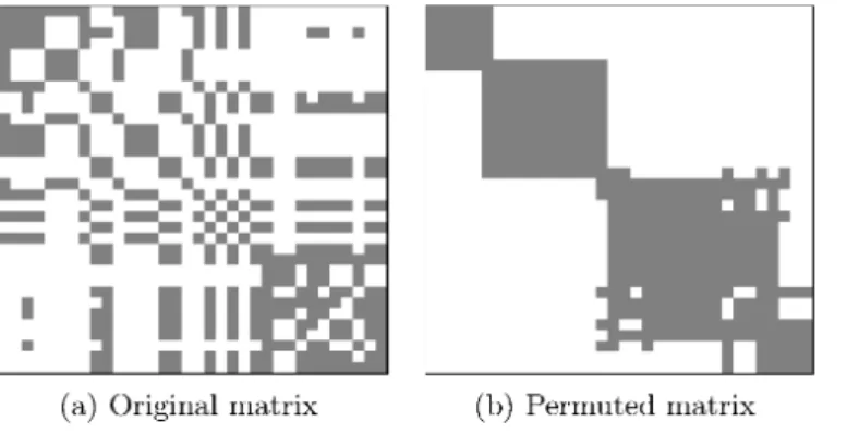
non-increasing order of values of components of $u^{2}$. Take a benchmark instance Karate for

example, we show an optimal solution $Z^{*}$ ofDNN and the matrix obtained in the

manner

described above in Figures 1 (a) and (b). $Rom$_{these figures,} we observe that the permuted

1

1

I

$\ovalbox{\tt\small REJECT}$

..

(a) Original matrix (b) Permuted matrix

matrix is considerably close to a block diagonal matrix. However, there is no theoretical

validity of using the eigenvector corresponding to the second largest eigenvalue. Here still

remains room for further research.

6.2. Dynamic programming. Next, we discuss how to construct a feasible solution of MD from the permuted matrix. Let $\overline{V}$

be a sequence of nodes consistent with the

non-increasing order of components of$u^{2}$. For the sake

of notational simplicity, we renumber the nodes in $V$ and denote the sequence $\overline{V}$

by $(1, 2, \ldots, n)$. Now, we try to find a _partition

with maximum modularity density of $\overline{V}$

under the constraint that each member consists of consecutive indices of$\overline{V}$

. For this problem, we propose an algorithm using the dynamic programming. We define $q(k, l)$ by

$q(k, l)= \frac{2\sum_{i=k}^{l}\sum_{j=k}^{l}a_{ij}-\sum_{i=k}^{l}d_{i}}{l-(k-1)}$

for $k$ and $l$ of $\overline{V}$

with $k\leq l$

.

The value$q(k, l)$ represents the contribution ofthe community

$(k, \ldots, l)$ of $\overline{V}$

to the modularity density when it is selected as a member of the partition. For any index $s$ of

$\overline{V}$

, let $\mu(s)$ be the maximum modularity density that is achieved by

partitioning the sequence $(1, \ldots, s)$ into several consecutive subsequences. If we define

$\mu(0)=0$ for notational convenience, then $\mu(s)$ satisfies the recursive equation

$\mu(s)=\max\{\mu(h)+q(h+1, s)|h\in\{0, 1, . . . , s-1\}\}$. (6.1) Owing to (6.1), starting from $\mu(1)=q(1,1)$, we first obtain

$\mu(2)=\max\{q(1,2), \mu(1)+q(2,2)\},$

then obtain $\mu(3)$ by means of$\mu(1)$ and $\mu(2)$, and so on. Our algorithm is given as follows.

AlgorithmDP

Step 1 : Solve the relaxation problem to obtain an optimal solution $Z^{*}.$

Step2 : Find the eigenvector $u^{2}$

corresponding to the second largest eigenvalue of $Z^{*}.$

Let $\overline{V}=(1,2, \ldots, n)$ be asequence of nodes obtained by rearranging them in

non-increasing order of corresponding components in $u^{2}.$

Step3 : Set $\mu(O)$ $:=0.$

for $s=1$ to $n$ do

Compute $\mu(s)$ accordingto (6.1).

end-do

7. COMPUTATIONAL EXPERIMENTS

To evaluate the lower and upper bounds obtained by our algorithm, we conducted the computational experiments. The experiments

were

performed on a computer with Intel Corei7, 3.70 GHz processor and 32.0GB of memory. Using SeDuMil$.2$ as an SDP solver,

we implemented the algorithm in MATLAB 2010.

In the experiments,weusedseveninstances; Michael’s strike dataset [20], Zachary’skarate dataset [30], Gil-MendietaandSchmidt’s Mexicodataset [12], Michaeland Massey’s sawmill dataset [21], Lusseau’s dolphinsdataset [18], Hugo’s Les Mis\’erables dataset [14], and Krebs’ books dataset [15]. Details of each instance are listedinTable 1, where the columns $(LB^{\star}$”

and “‘$t^{\star}$”’ represent

respectively. Since the first fourinstances inthetablewere solved to optimalityin Costa [7], the optimal values and the optimal numbers of communities are listed. For the remaining instances,

we

list the lower bounds and the number ofcommunities reported in Costa $et$

al. [8] since the instances

were

not solved so far to

our

knowledge.

Table 1: Instances $\overline{\frac{IDnamenmLB^{\star}t^{\star}}{1Strike24388.86114}}$ $2$ Karate 34 78 7.8451 3 3 Mexico 35 117 8.7180 3 4 Sawmill 36 62 8.6233 4 5 Dolphins 62 159 12.1252 5 6 Les Mis\’erables 77 254 24.5339 9 7 Books 105 441

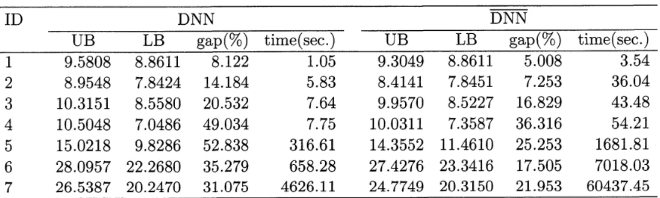
21.9652

7

Table 2 shows the computational results of the algorithm described in Subsection 6.2, where the columns “UB”, “LB”, “gap” and “time represent the optimal value of the relax-ation problem, the lower bound obtained by the algorithm DP, the duality gap defined by 100(UB–LB)/LB, and the computation time in seconds, respectively. For each instance,

we

observed that the predominant portion of the computation time

was

spent for solving

a relaxation problem, and the remaining parts of the algorithm require a fraction of time, specifically less than one second.

Table 2: Computational results of

our

algorithm

$\frac{ID\frac{DNN}{UBLBgap.(\%)time(se.c.)}\frac{\overline{DNN}}{UBLBgap.(\%)time(se.c.)}}{19.58088.861181221059.30498.86115008354}$ $2$ 8.9548 7.8424 14.184 5.83 8.4141 7.8451 7.253 36.04 3 10.3151 8.5580 20.532 7.64 9.9570 8.5227 16.829 43.48 4 10.5048 7.0486

49.034

7.75 10.0311 7.3587 36.316 54.21 5 15.0218

9.8286

52.838

316.61 14.3552 11.4610 25.253 1681.81 6 28.0957 22.2680 35.279 658.28 27.4276 23.3416 17.505 7018.03 7 26.5387 20.2470 31.075 4626.11 24.7749 20.3150 21.953 60437.45

From Table 2, we observe that the upper bounds UB provided by $\overline{DNN}$ are tighter than

those provided by DNN for all instances, which indicates the effectiveness of the valid in-equalities in Lemma5.1. Moreover, we also confirm that the lower bounds obtained for$\overline{DNN}$

are

equal toor larger than those obtained for DNN for all instances except Mexico $($ID$=3)$.

However, solvingtheproblem$\overline{DNN}$requires aratherlong computationtime comparedwith

solving DNN asthe instance sizegrows. To be specific, for the instance Books $($ID$=7)$, DNN takes approximately 4600 seconds, whereas DNN takes

over

60000 seconds, approximately

Table 3: Computational results of the branch-and-bound algorithm for MILP formulation $\frac{ID\frac{MILP}{8.86118.86110050UBLBgap(\%)time(se.c.)}}{1}$ $2$ 7.8451 7.8451 $0$ 0.74 3 8.7180 8.7180 $0$ 7.84 4 8.6233 8.6233 $0$ 6.10 5 13.8466 12.1252

14.196

86400.00

6 61.6302 24.5339 151.204 86400.00 7 54.6234 21.6803 151.949 86400.00

Next,

we

solve the problem MILP by branch-and-bound algorithm in Gurobi6.0.0 to

compare the quality of the solutions obtained by

our

algorithm for $0$-ISDP formulation.

The computationalresults aregiven in Table 3. Inour experiments, we impose a time limit

of86400 seconds, 24 hours, on the computation time of the branch-and-bound algorithm.

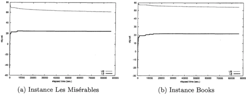
In Table 3, we see that the first four instances are solved to optimality within a short computation time, while the remaining instances cannot be solved within the time limit. Especially, for the instances Les Mis\’erables $($ID_$=6)$ and Books $($ID$=7)$, a quite large duality gap remains. Figures 2 (a) and (b) show the upper and lower bounds vs. the elapsed time. From the figures, we observe the following behavior: (i) the branch-and-bound algorithm

(a) Instance Les Mis\’erables (b) Instance Books

Figure 2: The upper and lower bounds vs. elapsed time in the branch-and-bound

gives a good lower bound in early stage, and (ii) the improvement of upper bound rarely

occurs

throughout the computation. Owing to the latter of these, the duality gap still

remains large

even

though a good feasible solution has been found. This suggests that deriving a tight upper bound enables us to estimate the accuracy of

an

incumbent solution obtained by the branch-and-bound algorithm more precisely.

8. CONCLUSION

Inthis paper, wepresented$0$-ISDP formulationoriginallyintroducedby PengandXia [25]

theproblem$0$-ISDP and themodularitydensitymaximization. Then,weproposedamethod

to solve adoubly non-negative relaxation of theproblem$0$-ISDP inorder to obtain anupper

bound

on

the modularity density. The advantage ofthe relaxation problem is twofold: the problemdoes not require the number of communities be known, and the size of the problem depends on neither the number of communities nor the number of edges. In addition, we

developed

a

lower bounding algorithm based on the combination of spectral heuristics and dynamic programming.

The relaxation problem for

our

formulation

was

numerically compared to MILP formu-lation, and the results showed that the upper bounds provided by our formulation are

competitive.

We observed that the solution matrix showed a block-diagonal-like structure when its

rows and columns are rearranged simultaneously in accordance with the magnitude ofthe components ofthe eigenvector corresponding to the second largest eigenvalue. Theoretical study should be carried out about whether this procedure functions effectively, and why if it does. The alternative to form

a

block-diagonal-like matrix is to develop

a

heuristics based on the numerical linear algebraic computation such

as

the algorithms of Sargent and Westerberg [26], and Tarjan [27].

REFERENCES

[1] T. Achterberg. SCIP: Solving constraint integer programs. Mathematical Programming Computation, 1(1):1-41, 2009.

[2] G. Agarwal and D. Kempe. Modularity-maximizing graph communities via mathematical programming.

The EuropeanPhysical JournalB, $66(3):409-418$, 2008.

[3] D. Aloise, S. Cafieri, G. Caporossi, P. Hansen, S. Perron, and L. Liberti. Columngenerationalgorithms

for exact modularity maximizationin networks. Physical ReviewE, $82(4):046112$, 2010.

[4] A. Arenas, A. Fern\’andez, and S. G\’omez. Analysis of the structure of complex networks at different resolution levels. NewJournal _ofPhysics, $10(5):053039$, 2008.

[5] H.P. Benson. Global optimization algorithm for thenonlinear sum of ratios problem. Journal

_of

Opti-mization Theory and Applications, $112(1):1-29$, 2002.

[6] U. Brandes, D. Delling, M. Gaertler, R. Gorke,M. Hoefer,Z. Nikoloski, and D. Wagner. Onmodularity

clustering. IEEE Transactions on Knowledge and Data Engineenng, $20(2):172-188$, 2008.

[7] A. Costa. MILP formulations for the modularity density maximization problem. European Journal _of Operational Research, $245(1):14-21$, 2015.

[8] A. Costa,S. Kushnarev, L. Liberti, and Z. Sun.Divisive heuristic for modularity density maximization. optimization Online, 2015. http:$//www$._{optimization online.}$org/DB_{-}HTML/2015/09/5116$.html.

[9] W. Dinkelbach. On nonlinear fractional programming. ManagementScience, $13(7):492-498$, 1967.

[10] R. Fortet. Applications de lalgebre de boole en recherche op\’erationelle. Revue Frangaise de Recherche Op\’erationelle,$4(14):17-26$, 1960.

[11] S. Fortunato and M. Barth\’elemy. Resolution limit in communitydetection. Proceedings ofthe National

Academy_ofSciences, 104(1):36-41, 2007.

[12] J.Gil-MendietaandS. Schmidt. The political network in mexico. SocialNetworks, $18(4):355-381$, 1996. [13] C. Granell, S. Gomez, and A. Arenas. Hierarchical multiresolution methodtoovercome the resolution

limit incomplex networks. International Journal of Bifurcation and Chaos, $22(7):1250171$, 2012. [14] D.E. Knuth. The _Stanford GraphBase: A platformfor combinatorial computing, volume 37.

Addison-Wesley Reading, 1993.

[15] V Krebs. http:$//www$._orgnet.$com/($_{last visited october 13,} 2015

[16] T. Kuno. A branch-and-bound algorithm for maximizing the sum of several linear ratios. Journal _of

Global optimization, $22(1-4):155-174$, 2002.

[17] Z. Li, S. Zhang, R.S. Wang, X.S. Zhang, and L. Chen. Quantitative function for community detection.

[18] D. Lusseau, K. Schneider, O.J.Boisseau, P. Haase, E. Slooten, andS.M. Dawson.Thebottlenosedolphin communityofdoubtfulsoundfeaturesalarge proportion of long-lasting associations. Behavioral Ecology andSociobiology, 54(4):396-405, 2003.

[19] G.P. McCormick. Computability of global solutions to factorable nonconvexprograms: Part I convex

underestimatingproblems. Mathematical Programming, 10(1):147-175, 1976.

[20] J.H. Michael. Labor disputereconciliation in a forest productsmanufacturing facility. Forest Products

Journal 47(11/12):41-45, 1997.

[21] J.H. Michael and J.G. Massey. Modeling the communication network in a sawmill. Forest Products

Journal,$47(9):25-30$, 1997.

[22] S. Muff, F. Rao, andA. Caflisch. Local modularitymeasurefor network clusterizations. PhysicalReview

E, $72(5):056107$, 2005.

[23] M.E. Newman. Fast algorithm for detecting community structure in networks. Physical Review E,

$69(6):066133$, 2004.

[24] M.E.NewmanandM.Girvan.Finding and evaluating communitystructurein networks. Physical Review E, $69(2):026113$, 2004.

[25] J. Peng and Y. Xia. A newtheoretical framework for $k$-meanstype clustering. In Studies in Fuzziness and _Soft Computing, volume 180, chapter Foundations and Advances in Data Mining, pages 79-96.

Springer, 2005.

[26] R.W.H. Sargent and A.W. Westerberg. Speed-up in chemical engineering design. Transactions _ofthe Institution _ofChemical Engineers, 42:190-197, 1964.

[27] R. Tarjan. Depth-first search and linear graph algorithms. SIAMJournal on Computing, 1(2):146-160,

1972.

[2S] V.A. Raag, P. Van Dooren, and Y. Nesterov. Narrow scope forresolution-limit-free community

detec-tion. PhysicalReviewE, $84(1):016114$, 2011.

[29] G. Xu, S. Tsoka, and L.G. Papageorgiou. Finding community structures in complex networks using

mixed integer optimisation. The EuropeanPhysical JournalB, $60(2):231-239$, 2007.

[30] W.W. Zachary. An informationflow model for conflict and fission in small groups. Journal _of

Anthro-pologicalResearch, 33(4):452-473, 1977.

(Y.Izunaga) GRADUATE SCHOOLOFSYSTEMSANDINFORMATION ENGINEERING, UNIVERSITYOFTSUKUBA, TSUKUBA, IBARAKI 305-8573, JAPAN

$E$-mailaddress: s1130131@sk.tsukuba.ac.jp

(T. Matsui) DEPARTMENT OF SOCIAL ENGINEERING, GRADUATE SCHOOL OF DECISION SCIENCE AND

TECHNOLOGY, TOKYO INSTITUTE OF TECHNOLOGY, MEGURO-KU, TOKYO 152-s550, JAPAN

$E$-mail address: _{mat sui.}$t$.af@m.titech.ac.jp

(Y. Yamamoto) FACULTY OF ENGINEERING, INFORMATION AND SYSTEMS, UNIVERSITY OF TSUKUBA,

TSUKUBA, IBARAKI 305-8573, JAPAN

$E$_{-mail address: yamamoto@sk.tsukuba.} ac.jp