Chaotic mixing due to a spatially periodic three-dimensional flow (Turbulence Transport, Diffusion and Mixing)

Chaotic mixing due

to

aspatially periodic three-dimensional

flow

京都大学大学院情報学研究科

水野吉規 (Yoshinori Mizuno), 船越満明 (Mitsuaki Funakoshi)

Graduate School ofInformatics, Kyoto University

1

Introduction

Mixing of afluid has been studied

on

the basis of theories of dynamical systems. It

is known that Stokes flow

or

aflow with low Reynolds numbers

can

mix the fluid well

within aregion where the trajectories of fluid particles

are

chaotic, called chaotic region

hereinafter,

even

if the velocity field itself behaves regularly

or

is steady if it is

thoee-dimensional (Ottino (1989), Ottino (1990) and Aref (1990)). Partitioned pipe mixer

(PPM) is one ofthe systems studied from the viewpoint of dynamical systems (Khakhar

et al. (1987), Ling (1993) and Meleshko et al. (1999)$)$

.

This system first introduced by

Khakhar et al. originally consists of

an

infinitely long cylinder and plane plates ofthe

same

length fixed orthogonally

to

each other. Figure $1(\mathrm{a})$ shows schematic view of

one

period of the original PPM. Rotation ofthe cylindrical wall and pressure gradient in the

axial direction

cause

aflow in this system. In Khakhar et al. (1987) and Meleshko et al.

(1999) that

are

based

on

approximate velocity fields, it is shown that chaotic mixing

can

occur

inthis system. Mizuno and Funakoshi (2002) thengeneralizedthe PPM

so

thatthe

ratio of the lengths of neighboringplates

or

the angle between them

can

bechanged. One

period ofthe generalized PPM is shown in Fig.l(b). Inthe examination of the mixing of

afluid within the generalized PPM, it is shown that the chaotic region

can

occupy the

$\backslash$

almost whole region ifthe ratio or the angle is appropriately changed.

Generally, there exists regions that donot mix quickly with the surrounding fluid

even

within chaotic regions. It is confirmed by calculating the distribution of stretching rate

offluid elements(Muzzio et al. (1991)). Capturing theexistenceand distribution of these

regions needs to understand the mixing process there. In the experimental study

on

the

mixing in PPM by Kusch and Ottino (1992), it

was

noted that the separation of the

fluid by the leading edges of plane plates is acontributing mechanism to the mixing.

Although they also noted that chaos

can

occur

without anycutting mechanism, the

con-sideration of this mechanism which static mixers commonly possess is expected to be

a

useful approach to understanding the mixing process in these mixers. Hence, Mizuno

and Funakoshi (2002) focused

on

the separation of the flow by the leading edges, and

examined the efficiency of the mixing within the chaotic region by introducing the lines

of

separation, defined

as

the set of

cross-

ectional initial locations of fluid particles which

move

to

one

of the leading edges of the plates within aspecified period. Consequently,

it

was

found that the lnes ofseparationplays

an

important role in the estimation ofthe

数理解析研究所講究録 1339 巻 2003 年 23-34

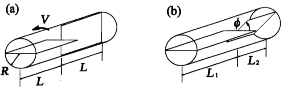
Figure 1: Schematic view ofPPMs. (a) Original PPM. (b) Generalized PPM.

mixing performance inafew periods.

However,it should benoted that thevelocityfieldsin the precedingstudies

are

assumed

tobe independent of theaxial coordinatewithineachregionaround each plate, hereinafter

an

element, and to change discontinuously at the cross-sections between neighboring

el-ements. The validity of these assumptions is not clear. Therefore,

we

here calculate the

velocityfield numerically without these assumptions, and examine the mixing of afluid,

especially in

one

period. Furthermore,

we

will show that the consideration of the

sep-aration by the leading edges help to understand the mixing process within the chaotic

region.

2Velocity field in PPM

Let $(r, \theta)$ be the polar coordinates in the cross-sectional direction of

aPiPe

with radius

$R$, and $z$ be the coordinate in its axial direction. The cylindrical $\mathrm{w}\mathrm{a}\mathrm{U}r$ $=R$ of the pipe

is assumed to rotate at constant velocity $V$. Horizontal platesof length $L_{1}$ expressed by

{

$(r,\theta,z)|0\leq r\leq R$, $\theta=0$

or

$\pi$, $k(L_{1}+L_{2})<z$ $<k(L_{1}+L_{2})+L_{1}$

}

and verticalplates

oflength $L_{2}$ expressed by

{

$(r,\theta,z)$ $|0\leq r\leq R$

,

$\theta=\pi/2$

or

$3\pi/2$, $k(L_{1}+L_{2})+L_{1}<z$ $<$

$(k +1)(L_{1}+L_{2})\}$

are

placed alternatelywithin this pipe, where A $=0,$$\pm 1,$$\pm 2$,$\cdots$

.

Assuming the spatial periodicity in the axial directionof the system,

we

take the flow

region

as

$\mathrm{D}=\{(r,\theta,z)|0<r<R, 0<\theta<2\pi, : 0<z<L_{1}+L_{2}\}$

.

We here

assume

the steady Stokes flow in region D. If the velocity field and pressure

are

$v=(v_{r}, v_{\theta},v_{z})$ and $P$, respectively, the equation of continuity and the $\mathrm{N}\mathrm{a}\mathrm{v}\mathrm{i}\mathrm{e}\mathrm{r}\sim \mathrm{S}\mathrm{t}\mathrm{o}\mathrm{k}\mathrm{s}$

equation under the Stokes approximation

are

given by

$\nabla\cdot v=0$, (1)

$- \frac{\partial P}{\partial r}+\beta(\frac{\partial^{2}v_{r}}{\partial r^{2}}+\frac{1}{r}\frac{\partial v_{r}}{\partial r}+\frac{1}{r^{2}}\frac{\partial^{2}v_{r}}{\partial\theta^{2}}+\alpha^{2}\frac{\partial^{2}v_{r}}{\partial z^{2}}-\frac{v_{r}}{r^{2}}-\frac{2\partial v_{\theta}}{r^{2}\partial\theta})=0$

,

(2)

$- \frac{1}{r}\frac{\partial P}{\partial\theta}+\beta(\frac{\partial^{2}v_{\theta}}{\partial r^{2}}+\frac{1}{r}\frac{\partial v_{\theta}}{\partial r}+\frac{1}{r^{2}}\frac{\partial^{2}v_{\theta}}{\partial\theta^{2}}+\alpha^{2}\frac{\partial^{2}v_{\theta}}{\partial z^{2}}-\frac{v_{\theta}}{r^{2}}+\frac{2}{r^{2}}\frac{\partial v_{r}}{\partial\theta})=0$,

$- \alpha^{2}\frac{\partial P}{\partial z}+\beta(\frac{\partial^{2}v_{z}}{\partial r^{2}}+\frac{1}{r}\frac{\partial v_{z}}{\partial r}+\frac{1}{r^{2}}\frac{\partial^{2}v_{z}}{\partial\theta^{2}}+\alpha^{2}\frac{\partial^{2}v_{z}}{\partial z^{2}})=0$,

(3) (4) $v=0$

on

$\{$ $\theta=0,\pi$, $0<z<l_{1}$, $\theta=\frac{\pi}{2}$,$\frac{3\pi}{2}$

,

$l_{1}<z<2$, (5) $v_{r},v_{z}=0$, $v_{\theta}=1$

on

$r=1$, (6) $v(z=0)=v(z=2)$

,

$P(z=0)=P(z=2)+1$, (7) where

$\alpha=\frac{R}{(L_{1}+L_{2})/2}$, $\beta=\frac{\mu V}{RP_{d}}$, $l_{1}= \frac{L_{1}}{(L_{1}+L_{2})/2}$,

and

we

non-dimensionalized thelength in the cross-sectionaldirection, length inthe axial

direction,

velocities

in the cross-sectional direction, velocity in the axial direction and

pressure with $R$, $(L_{1}+L_{2})/2$, $V$, $(L/R)V$ and $P_{d}$, respectively. Here $\mu$ and $P_{d}$

are

the

viscosity of the fluid and the pressure drop during

one

period in the axial direction,

respectively. The parameter $\alpha$ is the aspect ratio ofthe system, and $\beta$ is the ratio ofthe

representative velocity of the cross-sectional flow due to the rotation of the cylindrical wall to that of the axial flow due to the pressure gradient.

The boundary value problem (1)$-(7)$ is solved numerically. We here assume that the

velocity and pressure fields have the symmetry with respect to the rotation by $\pi$ around

the $z$ axis. Hence,

we

restrict the range of

0to

$(0, \pi)$

.

Since the velocity field changes

largely in the regions around $z=0$, $l_{1}$ and 2,

we

use

acoordinate $\langle$ that is stretched

within these regions instead of$z$

.

The relation between $z$ and $\langle$ is given by

$z=\{pq\{$$\{$

$\frac{1}{2}+\epsilon)\pi\zeta-\frac{1}{2}$$\mathrm{c}\mathrm{o}\mathrm{e}(\pi\zeta)$$\sin(\pi\zeta)\}$, $0<\zeta<1$ $\frac{1}{2}+\epsilon\frac{p}{q})\pi(\zeta-1)-\frac{1}{2}\cos(\pi(\zeta-1))\sin(\pi(\zeta-1))\}+l_{1}$, _$1<\zeta<2$,

(8)

where

$p= \frac{l_{1}}{\pi/2+\epsilon\pi}$, $q= \frac{2-l_{1}+4\epsilon(1-l_{1})}{\pi/2+\epsilon\pi}$,

and $\epsilon$ is

anon-zero

value chosen

so

that $| \frac{\ }{d\zeta}|\neq 0$ at ( $=0,1,2$

.

We choose $\epsilon=0.5$ for

$a=1.0$, $\epsilon=0.3$ for $a=1.85,2.33$

,

and $\epsilon=0.2$ for $a=3.0$

.

We obtain the velocityfield

satisfying Eqs.(1)-(7)

as

the steady solution to

$\nabla\cdot$ $v=0$, and, $\frac{\partial v}{\partial t}=-\mathrm{f}\mathrm{f}\mathrm{f}\mathrm{f}\mathrm{i}P$$+\beta\nabla^{2}v$, (9)

with boundary conditions (5)$-(7)$ by

SMAC

method (Ferziger and Peric (1999)) with

fi-nite difference method

on

astaggered grid. The accuracy of the discretization is

secon

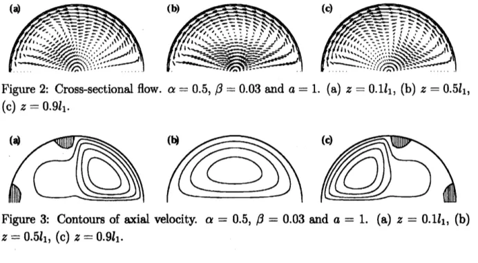
Figure 2: Cross-sectional flow, $\alpha=0.5$, $\beta=0.03$ and $a=1$

.

(a) $z=0.1l_{1_{7}}(\mathrm{b})z=0.5l_{1}$,

(c) $z=0.9l_{1}$

.

Figure 3: Contours of axial velocity, $\alpha=0.5$, _$\beta=0.03$ and _$a=1$

.

(a) $z=0.1l_{1}$, (b)

$z=0.5l_{1}$, (c) $z$ $=0.9l_{1}$

.

order, and the number of the grid points is 40 $\mathrm{x}40\mathrm{x}80$

.

The cross-sectional flow and contours ofthe axial velocity at three axial positions

are

shown in Figs.2 and 3, respectively. Only the upper parts

are

shown in these figures.

The wall rotation generates vortical flows in the cross-sectional direction at all the axial

positions, as seenin Fig.2. In the axialdirection, althoughtotalfluxispositivebecause of

the pressure drop inthe axial direction,

we

can

recognize backward flows

near

the ends of

the plate,

as

shown in Figs.3(a) and (c), where backward flows

occur

within the hatched

regions. These backwardflows

are

caused bythe wall rotation. Incontrast to the

approx-imate velocityfields used in the precedingstudies, there

can

be orbits wandering between

neighboring elements for along time and also closed orbits because of the backwardflow.

Although the former orbits

are

chaotic, they stay within apair of neighboring elements

for along time. Since such orbits are not appropriate for amixing device,

we

choose the

smal value of$\beta$

so

that the region in which the axial velocity has backward direction is

small. Backward flow was also observed in the experimental study by Kusch and Ottino

(1992).

3Results

Once avelocity field is obtained,

we can

track the trajectories of fluid particles by

integrating ordinary differential equation

$\frac{dx(t)}{dt}=v(x(t))$, (10)

where $x(t)$ is the position of afluid particle, and t is the time non-dimensionalized by

$R/V$

.

Since the velocity is periodic in the axial direction,

we

here consider amap defined

as

$M_{z_{0}}$ : $(r,\theta)\mapsto(r(T(r,\ )), \theta(T(r,\theta)))$, (11)

where $T(r, \theta)$ is the minimum time which satisfies

$\int_{0}^{T(r\beta)}v_{z}(t)dt.=2$, (12)

on

thetrajectoryofEq.(lO) starting from $(r, \theta, z_{0})$ at $t=0$

.

This mapping represents the

cross-sectional movement ofthe fluid particle initiallylocated at $(r, \theta)$

on

_{$z=z_{0}$} after

one

period in the axial direction, and $T(r,\theta)$ is the time required for the movement.

3.1

Poincare

sections

In the preceding studies based

on

the approximate velocityfield andalso in the

exper-imental study, tubular invariant sets of the trajectories, called KAM-tubes hereinafter,

that prevent thetransport of fluidparticlesbetweenitsinside and outside

were

recognized

for

some

sets of the values of system parameters. We

can

also find them in Poincare’

sec-tions based

on

the numerically obtained velocity field. The Poincare sections associated

with $\mathrm{M}\mathrm{j}\mathrm{i}/2$for three values of$\beta$ with $\alpha$and $a$ fixed to 0.5 and 1.0, respectively,

are

shown

in Fig.4. It is found that the islands

can

shrink

or

disappear

as

$\beta$ increases. Figures

5and 6show the Poincare sections for three values of $a$ with

4fixed

to 0.01 and 0.03,

respectively. For $\beta=0.01$, some islands disappear

as

$a$ increases from 1.0. However,

other islandsremainand become larger. On the otherhand, for $\beta$ $=0.03$, norecognizable

island exists for $a=2.33$ and 3.0 although weobserve afew islands for $a=1.0$,

as

shown

in Fig.6. This shows that changing $a$

can erase

the KAM-tubes for appropriate values of

$\beta$

.

Although understanding the mixing process within chaotic region is also important

is-sue

for applications,

we

cannot obtain information

on

it from these Poincare’ sections.

Therefore,

we

next examine the mixing process within the chaotic region by introducing

the lines of separation.

3.2

Lines of

separation

and

mixing

process

in chaotic region

We introduce the lines of separation, $U_{z\mathrm{o}}^{\mathrm{n}}$, in order to examine the mixing ofafluid in

the chaotic region. Before giving the definition of the lines of separation,

we

introduce

(a) (b) (c)

Figure 4: Poincar\’e sections based

on

$M_{l_{1}/2}$

.

$\alpha=0.5$ and $a=1.\mathrm{O}$

.

(a) $\beta=0.01$

,

(b)

$\beta=0.03$, (c) $\beta=0.1.83$ fluid particles

are

initiaUy placed

on

square grid points of

(a) (b) (c)

Figure 5: Poincare sections based

on

$M_{l_{1}/2}$

.

$\alpha=0.5$ and $/\mathit{3}=0.01$

.

(a) $a=1.85$, (b)

$a=2.33$, (c) $a=3.0$

.

The initial locations offluid particles and the period of plotting

(a) (b) (c)

Figure 6: Poincare’ sections based

on

$M_{l_{1}/2}$

.

$at=0.5$ and $\beta=0.03$

.

(a) $a=1.85$, (b)

$a=2.33$, (c) $a=3.0$

.

The initial locations of fluid particles and the period of plotting

are

the

same as

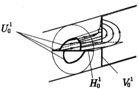
Fig.4.

$U_{0}^{1}$

Figure 7: Aschematic view of the lines ofseparation, $U_{0}^{1}$

.

two sets:

$H_{z_{\mathrm{O}}}^{n}=\{(r,\theta,z)|0<r<1,\theta=0,\pi,z =2,4, \cdots,2n\}$, (13)

$V_{z_{\mathrm{O}}}^{n}=\{\begin{array}{l}\{(r,\theta,z)|0<\mathrm{r}<1,\theta=\frac{\pi}{2},\frac{3\pi}{2},z=l_{1},l_{1}+2,\cdots,l_{1}+2(n-1)\}\mathrm{f}\mathrm{o}\mathrm{r}\mathrm{a}<l_{1}\{(r,\theta,z)|0<r<1,\theta=\frac{\pi}{2}\frac{3\pi}{2}z=l_{1},l_{1}+2,\cdots,l_{1}+2n\}\mathrm{f}\mathrm{o}\mathrm{r}\mathrm{a}>l_{1}\end{array}$ (14)

These

are

the positions of the leading edges of horizontal and vertical plates within $n$

periods from $z=z_{0}$

.

Then, we define the lines of separation, $U_{z0}^{n}$, as

$U_{z_{0}}^{\mathfrak{n}}= \{(r,\theta)|\lim_{tarrow\infty}x(t)\in H_{z_{0}}^{n}$

or

$V_{z_{0}}^{n}$

,

$x(0)=(r,\theta,\triangleleft)$,$z(t)\neq\hslash$for$t>0\}$

.

(13)

Hence,thefluid particles starting ffom$U_{z_{\mathrm{O}}}^{n}$reach

one

oftheleadingedges in$n$periods&0m

$z=\triangleleft$

.

Aschematic view of the lines of separation is given in Fig.7. In principle, exact

numerical calculation of $U_{z_{0}}^{\mathfrak{n}}$ is impossible because it needs to take the lmit of $tarrow\infty$

.

Here

we

calculate it approximately by integratingEq.(lO) inbackward time direction from

the Hues located slightlyapart from the leading edges, and collecting the cross-sectional

positions of them at $z=z_{0}$

.

In this way,

we

need to restrict the calculation time to

a

finite value $T_{\omega l}$ since thereexist particles which cannot reach at _$z=\alpha$ in afinite time.

We here choose $T_{\varpi l}=30$

.

Figure 8shows the lines ofseparation $U_{l_{1}/2}^{1}$ for

some

sets of

values of parameters. Fromthe definition, theends ofaline of separation

are

attached to

the cylindricalwall, aplane plate

or

another line of separation. Furthermore, the Hues do

not

cross

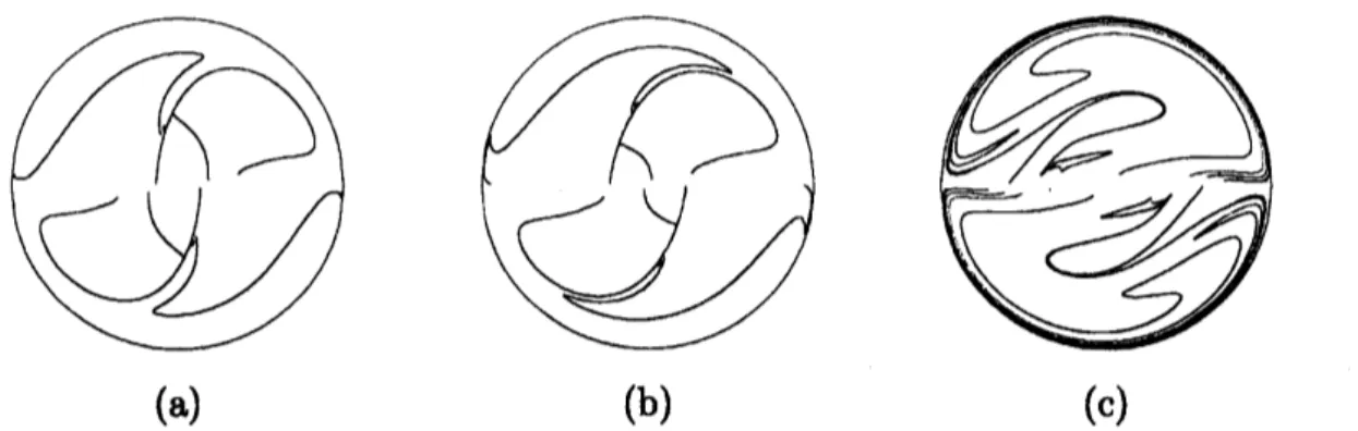
each other. However the lines in Fig.8 do not satisfy these conditions strictly

becauseofthe finite calculation time. The total lengthofthese lines

grows as

4increases,

because the effect of the wall rotation become stronger

as

$\beta$ increases, and then fluid is

stretched

more

strongly in the cross-sectional direction. Furthermore, by comparing the

distribution of the lines ofseparationwiththe corresponding Poincare sections,it isfound

that the lines exist only within the chaotic region. The

reason

for it is that islands

on

which map $M_{z_{0}}$ should be continuous cannot contain the lines of separation because the

map is discontinuous

on

them

(a) (b) (c)

Figure 8: Lines of separation, $U_{l_{1}/2}^{1}$

.

$\alpha=0.5$

.

(a) $\beta=0.01$, $a=1.\mathrm{O}$

,

(b) $\beta=0.01$

,

$a=1.85$, (c) $\beta=0.03$

,

$a=1.85$

.

The initial positions of

40000

trajectories calculated

here

are

uniformly placed

on

the lines 10 upstream from the leading edges.

We

can

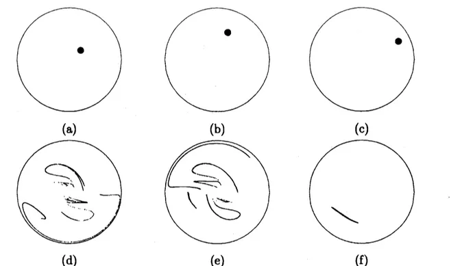
recognize the close relation between the stretching of fluid elements and the

lines of separation. Figure 9shows the initial locations of blobs

on

$z=l_{1}/2$ and their

evolutionsin

one

period. Blobs whose initiallocations

are

close tothe lines ofseparation,

such

as

Figs.9(a) and (b),

are

stronglystretched,whereas the blobs whose initial locations

axe

not close to them, such

as

Fig.9(c),

are

only weakly stretched. We obtained the

similar results in the calculations for different initial locations of blobs and the values of

the parameters. Hence, we can conclude that only the blobs starting from the vicinity of

the lines of separation

are

strongly stretched. Therefore, the separation by the leading

edges ofplates plays

an

important role in the mixing in PPM. The

reason

for the strong

stretching ofafluid inthe vicinity of the lines ofseparation is that theypass the regions

of large strain rate along the cylindrical $\mathrm{w}\mathrm{a}\mathrm{I}$ after the separation byaleading edge.

Khakhar et al. (1987) examined the residence time of each fluid particle defined

as

the time required for its movement

over

aspecific period for the original PPM using

the approximate velocity field, and found that the time ofparticles within the islands is

usually considerably smaller than that ofparticles within the chaotic region. Although

they considered the residence time for 5periods,

we

here calculate theresidence timesfor

only

one

period, that is $T(r, \theta)$ in Eq.(ll), in order to examine their distribution within

the chaotic region. Since the residence time of particles which pass very close to the

rigid wall and wandering between neighboring elements due to the backward flow

can

be infinite,

we

consider only the residence time $T$ satisfying $T<30$

.

Figure 10 shows

the contours of the residence time of particles whose initial positions

are on

$z=l_{1}/2$

.

The residencetime takes relatively largevalues in the regionswhere the contours densely

exist. From the comparisonbetween this figure and Fig.8,

we

find that the residencetime

is large around the lines of separation. The

reason

for it is that afluid particle starting

from the position

near

the lines of separation travels slowly in the axial direction since

they

move

along the rigid wall after passing by aleading edge. There is

no

difference

in the residence time distribution between the islands and the chaotic region. The larg

(c)

(d) (e) (f)

Figure

9:

Time evolution of small blobs. Each blob has radius 0.06. $\alpha=0.5$, $\beta=0.03$

,

and $a=1.\mathrm{O}$

.

Blobs in (a) and (b) which

axe

close to the lines ofseparation and that in

(c) which is not close to the lines evolve to (d), (e) and (f), respectively.

difference in the residence time between islands and the chaotic region,

seen

in Khakhar

et al. (1987)

seems

to be because they considered the residence time for 5periods which

is long enough for the lines ofseparation to spread

over

the chaotic region.

Finally,

we

shall

see some

numerical simulations of the time evolution of the dye

injected constantly at the fixed location on $z=z_{0}$

.

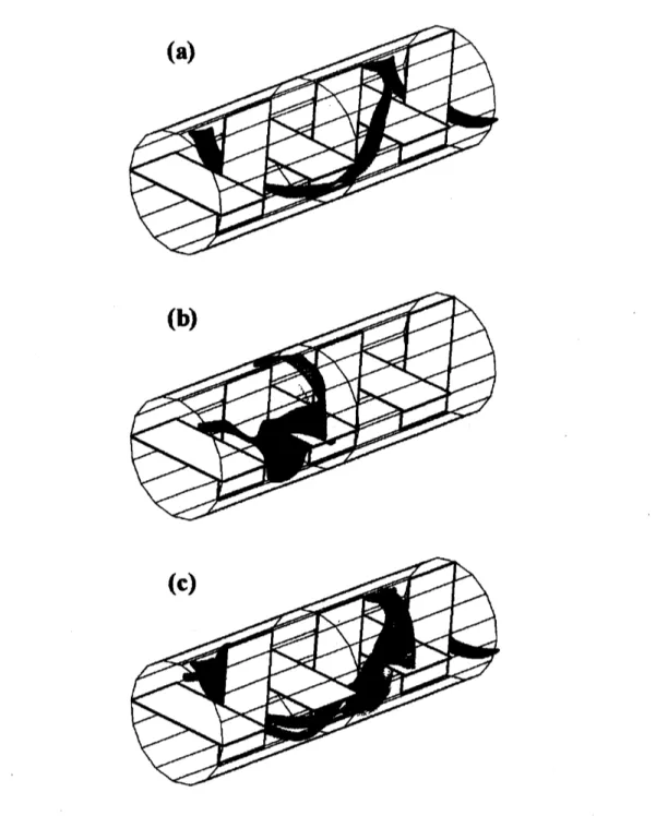
Figure ll(a) shows the dye streak

initially injected within aKAM-tube. We

see

that the dye travels in the axial direction,

staying inside the tube. Because the period of the stable periodic orbit which

cause

the

tube is 2, the streak

comes

back to the injected position after 2period. The dye streak

initiallyinjectedon $U_{l_{1}/2}^{1}$isshowninFig.ll(b). Thedye isonlyslightly stretched untilitis

Figure 10: Contours of the residence time based

on

the 98500 trajectories starting from

theinitialpositions

on

$z=l_{1}/2$

.

Theinitialpositions

are on

squaregridpoints ofinterval

0.01

on

the upper part ofthe cross-section, $\alpha=0.5$

.

(a) $\beta=0.01$, $a=1$, (b) $\beta=0.01$,

$a=1.85$, (c) $\beta=0.03$, $a=1.85$,

separated by the first leading edgeof the horizontalplate. After the separation, it travels

slowly along theplate, and thenis strongly stretchedinthe cross-sectionaldirection along

the cylindrical wall. In Fig.ll(c), the dye streak (grey) within the chaotic region whose

injected position is not close to $U_{l_{1}/2}^{1}$ and the streak (black) within the KAM-t be are

shown together. The grey dye travels in the axial direction without strong stretching

as

well as the black dye. The difference between their evolutions arises when the grey dye

is suddenly stretched after the separation by the leading edge of the second horizontal

plate. Theseobservations confirm the close relation between the mixing within the chaotic

region and the lines of separation.

4Conclusions

We numerically calculated the exact velocity field of the PPM system, and examined

the mixing ofafluid in this system. We thenfound that increasingtherelative strength,

$\beta$, of the wallrotation to that ofpressure gradient in the axial direction

or

changing the

ratio, $a$, of the lengthsof neighboring plates

can

shrink

or erase

tubular invariant sets of

trajectories which is amajor obstacle to the mixing. This result qualitatively coincides

with that in the previous studies.

Furthermore,

we

examined the mixing process within the chaotic region, byintroducing

the lnesof separation similarly to Mizuno and Funakoshi (2002). From the facts that

a

blob initialy close to the lnes of separation is strongly stretched in the

cross-

ectional

direction after it is separated by aleading edge and that only the regions of large strain

rate near the cylindrical wall contributes the stretching in the cross-sectional direction,

we can

expect efficient mixing in afew periods within the chaotic region wherethe lines

ofseparation for the correspondingperiods spread

over.

On the residencetimeoffluidparticles, Khakharet al. (1987) found that fluidparticles

within the tubular invariant sets travels in the axial direction relatively faster than the

particles outside them by calculating the residence time for 5periods. We here examined

their distributionwithin chaotic region, considering only

one

period. Wethen found that

the residence time for particles starting fromavicinity ofthe lines ofseparationis longer

than those for the initial positions located apart from the lines of separation. Provided

that the lines ofseparation spread

over

the chaotic region if theconsidered number of the

periods, $n$, is large enough, we expect to obtain the same distribution as in Khakhar et

al..

From the observation ofthe timeevolutionof the dyesfordifferent initialpositions,

we

found that fluid inside of KAM-tubes and fluid whose initial position is not close to the

lines of separation make the similar motion, that is, fast traveling in

the axial

direction

without strong stretching in the cross-sectional direction. The difference is that fluid

Figure 11: Dye streaks for different initial positions on $z=l_{1}/2$

.

$\alpha=0.5$, $\beta=0.03\mathrm{m}\mathrm{d}$ $a=1.\mathrm{O}$

.

Each blob is injected constantly at each initial position since$t=0.600$ particles

approximatingeachdye

are

initially placed within thecircle of radius0.06 centeredat (a) $(r\cos\theta,r\sin\theta)=(0,0.75)$, (b) (0, 0.4), (c) (-0.35, 0.5). (a) is the dye streak at $t=20$

injected within aKAM-tube. (b) is the dye streak at $t=10$ injected

on

$U_{l_{1}/2}^{1}$

.

(c) is the

dye streak (grey) at $t=16$ injectedwithin the chaotic region not

on

$U_{l_{1}/2}^{1}$

,

whichisshown

withthe

streak

(black) in (a)

elements within the chaotic region

are

suddenly stretchedjust after the separation by

a

leading edge.

References

Aref, H., 1990. Chaotic advection of

fluid

particles. Phil. Irans. R. Soc. Lond., A333,

273-288.

Ferziger, J.H. andPeric, M., 1999. Computationalmethods for fluid dynamics. Springer.

Franjione, J.G. and Ottino, J.M., 1992. Symmetryconcepts forthe geometric analysis of

mixing flows. Phil. Trans. R. Soc. Lond., A338, 301-323.

Khakhar, D.V., Franjione, J.G. and Ottino, J.M., 1987. Acase study of chaotic mixing

indeterministic flows: the partitioned-pipe mixer. Chem. Eng. Sci., 42, 2909-2926.

Kusch, H.A. and Ottino, J.M., 1992. Experiments

on

mixingin continuouschaotic flows.

J. Fluid Mech., 236,

319-348.

Ling, F.H., 1993. Chaotic mixing in aspatiallyperiodic continuous mixer. Phys. Fluids,

A5,

2147-2160.

Meleshko, V.V., Galaktionov, O.S., Peters, G.W.M. and Meijer, H.E.H., 1999.

Three-dimensional mixingin Stokes flow: the partitioned Pipe mixer problem revisited. Eur.

J. Mech. $\mathrm{B}/\mathrm{F}\mathrm{l}\mathrm{u}\mathrm{i}\mathrm{d}\mathrm{s}$, 18,

783-792.

Mizuno, Y. and Funakoshi, M., 2002. Chaotic mixing due to aspatially periodic

three-dimensional flow. FluidDyn. ${\rm Res}.$, 31, 129-149.

Muzzio, F.J., Swanson, P.D. and Ottino, J.M., 1991. The statistics of stretching and

stirring in chaotic flows. Phys. Fluids, A3, 822-834.

Ottino, J.M., 1989. The kinematics of mixing: stretching, chaos andtransport. Cambridge

University Press.

Ottino, J.M., 1990. Mixing, chaotic advection, and turbulence. Annu. Rev. Fluid Mech.,

22,

207-253