Abstract—It is important to know the spatial distributions of each climate element to evaluate local climate characteristics and long-term climate change on the Tibetan Plateau (TP) because of its huge area (about 2.5 × 10⁶ km2) and its complex terrain. We analyzed the monthly mean surface air temperature data of 90 meteorological stations from China Meteorological Administration on the TP. A linear model is used to examine the effects of altitude, latitude, longitude and other local environmental factors (valley, slope orientation, urban and other land use etc.) on the surface air temperature focusing on two periods: 1956-1980 and 1981-2005.
The linear model shows that surface air temperature decreases with increase of altitude, latitude and longitude. The model reveals that the lapse rate increased from 0.579ºC/100m for 1956-1980 to 0.594º C/100m for 1981-2005. This means that recent warming; especially warming in wintertime (when the lapse rate changed from 0.581º C/100m to 0.617ºC/100m) is clearer at lower altitude than at higher altitude. The study also shows that the latitude variation rate becomes smaller and longitude rate becomes greater in recent years,suggesting that the distribution of surface air temperature becomes less parallel to latitude and more parallel to longitude and that recent warming seems clearer in northwest part than in southeast part of the TP. The local environmental changes such as urbanization and land cove change may play very important role for the geographical changes of recent climate warming.
Keywords—Lapse rate, linear model, spatial pattern, surface air temperature.
I. INTRODUCTION
HE Tibetan plateau (TP) is generally defined as the regions above 3,000m ASL, which is the highest and largest plateau in the world. It has an average elevation of 4,000 m ASL and an area of about 2.5 × 10⁶ km2. The TP is characterized by This work was supported in part by the ‘Long-term monitoring on impacts of climate change in indicator ecosystems in terrestrial Asia’ project of the global environment research coordination system, Ministry of the Environment of Japan.
M. Du is with the Institute for Agro-Environmental Sciences, National Agriculture and Food Research Organization. Tsukuba, Ibaraki, 305-8604 Japan (Tel: +81-(0)298-38-8210, Fax: +81-(0)298-38-8199; e-mail:
J. Liu is with the Institute of Tibetan Plateau Research, Chinese Academy of Sciences. Beijing, 100085, China (e-mail: [email protected])
X. Zhang is with the Institute of Geographic Sciences and Natural Resources Research, Chinese Academy of Sciences, Beijing 100101, China (e-mail: [email protected])
Y. Li is with the Northwest Institute of Plateau Biology, Chinese Academy of Sciences, Xining 810001, China (e-mail: [email protected])
Y. Tang is with the College of Urban and Environmental Sciences, Peking University, China ([email protected])
complex terrain and 1/3 of the plateau is over 4800m. It is well known that the TP’s thermal and dynamical processes have a profound influence both to climate and to ecosystems of the Asian continent and even the whole world. Research on the climate and cryospheric change in the TP has received increasing attention since mid-1970s as [1] reviewed. Many works show that continuous warming has been taking place.
Furthermore, [2] showed that the main portion of the TP has experienced statistically significant warming since the mid-1950s, especially in winter, which exceed that of its surrounding regions and the warming rate rises with increasing altitude. Reference [3] shows that the warming rate increases from 3,000 to 4,800 m ASL, and then becomes quite stable with a slight decline near the highest altitude by using Moderate Resolution Imaging Spectroradiometer (MODIS) monthly averaged land surface temperature. However, [4] analyzed trend magnitudes of 11 indices of temperature extremes at 71 stations with elevations above 2000m ASL in the eastern and central Tibetan Plateau during 1961–2005 and failed to substantiate this relationship. Reference [4] pointed out that analysis of trend magnitudes by topographic type and degree of urbanization showed both factors to have a strong influence in the dataset, which overrides that of elevation. Therefore, spatial patterns should be considered due to its huge area (about 2.5 × 10⁶ km2) and its complex terrain. Although there have been considerable studies on physical-geographical elements of the TP as reviewed by [5], there is no model products or quantitative analyses to show their spatial distributions or patterns. This paper tries to get a linear model for showing the spatial distributions of surface air temperature and its change in recent years. Use this model and geographical information (latitude, longitude and altitude), one can get basic information of surface air temperature of TP.
II. DATA AND METHOD A. data
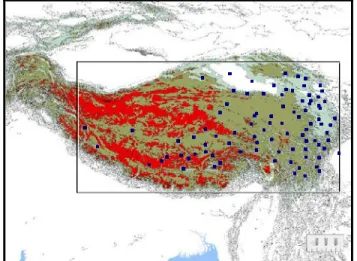
Fifty year’s monthly mean data from 1956 to 2005 of surface air temperature of most meteorological stations from China Meteorological Administration (CMA) on the TP are used in this study as shown in Fig.1. In order to clarify the change of the spatial patterns, we separate the 50 year’s time series into two 25 year’s periods as 1956-1980 and 1981-2005. In the first period 86 stations were used and in the second period 90 stations were used. 85 stations in both periods are used for
Spatial distributions of surface-air-temperature on the Tibetan Plateau and its recent changes
Mingyuan Du, Jingshi Liu, Xianzhou Zhang, Yingnian Li and Yanhong Tang
T
calculating the difference between the two periods.
Although the meteorological observatories on the TP are biased to the populated lower-elevation area (<4800m) in the eastern and southern TP and almost all the meteorological stations are located in valleys or basin bottoms as shown in Fig.
1, if we gridding the altitude data to draw a topography map by using all the stations’ altitude data, they still can represent the basic distribution of topography such as higher in the central and western part, big basin in the central north, some big valleys in the south eastern part, etc as show in Fig. 2. However, it cannot give any information above 4800m as shown in Fig. 2.
Fig. 1 Topography and location of the meteorological stations (black points and circles, the area of the square (80.08ºE -103.57ºE, 26.87-38.8ºN) was used for gridding).
Fig. 2 Topography deduced from meteorological station’s elevations by Kriging gridding method.
B. Linear model
In order to get the basic geographical features of mean surface air temperature, the following linear model is used:
T T
T T T T T T
cal
to la
al m a
∆ +
=
+ + + +
=
ln
(1)
where Ta, Tm, Tal, Tla, Tln and Tto are surface air temperature, regional mean surface air temperature, altitude deduce variation, latitude deduce variation, longitude deduced variation, and other topographical deduced variation, respectively. Tcal is
calculated surface air temperature from linear regression as below and ∆Tis the regression error. We assume this error is a worthwhile temperature, which is mainly deduced by local environmental factors (valley, slope orientation, urban and other land use, etc.) except altitude, latitude and longitude.
Thus,
dLn cLa bAl a
Tcal = + + + (2)
where Al, La and Ln are altitude, latitude and longitude respectively and a, b, c and d are regression coefficients.
Therefore, -b is lapse rate and -c, -d are variation rates (ºC/degree) for the latitude and longitude, respectively.
Using (1) and (2), we can remove the effects of latitude and longitude (adjust all the stations to a same latitude and longitude) to discuss the relation between surface air temperature and altitude and so to variation rates of the latitude and longitude.
In order to clarify the change of the spatial pattern, we calculated the mean monthly values and annual means of the two periods, 1956-1980 and 1981-2005. Using the model, we can get annual and 12 month’s regression functions by using SAS software (SAS institute inc., Cary, NC, USA) with t-test.
C. Gridding method
In order to draw the distribution map, we used the surface mapping system, Surfer software (Golden Software, Inc.
Calorado, USA). The Kriging gridding method was used.
III. RESULTS AND DISCUSSIONS A. Annual patterns
For anural mean air temperature, we get following model for the two periods.
39 . 1 151 . 0 813 . 0 00579 . 0 18 .
64 − − − ±
= Al La Ln
Tbefore (3)
39 . 1 182 . 0 772 . 0 00594 . 0 88 .
66 − − − ±
= Al La Ln
Tnow (4)
where Tbefore is the annual mean of surface air temperature for 1956-1980 and Tnow is that for 1981-2005.
It can be seen from (3) and (4) that the annual mean of surface air temperature decreasing with altitude, latitude and longitude increasing on the TP. The lapse rate is about 0.6ºC/100m. The decreasing rate with latitude is about 0.8ºC/degree and surface air temperature decreases about 0.2ºC with one-degree increase in longitude at same altitude and latitude. Using this model and geographical information (latitude, longitude and altitude), one can get the basic surface air temperature information with an error about 1.39ºC, which should be mainly effected by local topography, land use change and urbanization as discussed later.
B. Changes of annual means
Comparing (3) and (4), the lapse rate increased from
0.579ºC/100m for 1956-1980 to 0.594ºC/100m for 1981-2005.
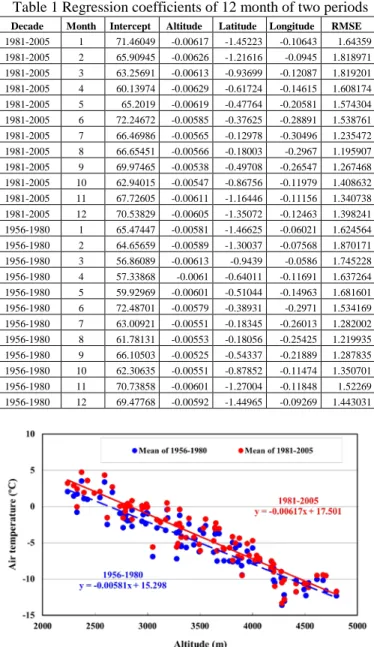
It seems that recent warming tended to be larger at lower altitude than at higher altitude. Using (3) and (4) to remove the effects of latitude and longitude, we can get the relationship between altitude and air temperature for the two periods as shown in Fig. 3. Although [2] has pointed that mean temperature rises in proportion to an increase in altitude in the TP, our model shows clearly the opposite results. This is because our model considered not only the altitude effect but also the effect of regional differences (latitude, longitude difference etc.). For example, from CMA data, annual surface air temperature at Caqia (3087.6m, 99°05'E, 36°47'N) was 1.54ºC before 1980 and changed to 1.95 now and annual surface air temperature at Damxung (4200m, 91°06'E, 30°29'N) was 1.31ºC before 1980 and changed to 1.84ºC now. Our model can evaluate these data as 1.4ºC, 2.1ºC for Caqia, and 1.3 and 1.82 for Damxung, respectively. As one cannot evaluate the lapse rate by dividing the temperature difference by the altitude deference (in this case, it will be about only 0.021ºC before 1980 and 0.0099ºC now), one cannot conclude that these warming, 0.41ºC at Caqia and 0.53ºC at Damxung by observation and 0.7ºC at Caqia and 0.52ºC at Damxung by our model, have any altitudinal dependence only by the two separated stations without consideration of regional differences.
Fig. 3 Relationship between annual mean of surface air temperature and altitude on the Tibetan Plateau of the two periods: before (1956-1980) and now (1981-2005). Latitude and longitude effects were removed by our linear model by adjusting all the station to the central part (91°06'E, 30°29'N)
Comparing (3) and (4), it can be seen that the latitude variation rate becomes smaller and longitude rate becomes greater in recent years. This means that the distribution of surface air temperature becomes less parallel to latitude and more parallel to longitude. Recent climate warming is clearer in northwest part than in southeast part of the TP. To verify the regional difference of climate warming on the TP, we calculated the differences of observational means between the two periods and the differences of our model results between the two periods.
Fig. 4 shows the distribution of the differences of the two datasets. It is clear that there is remarkable climate warming on the TP and the warming is clearer in northwestern part then in southeastern part except some small area. Our model shows the
regional differences more clearly. Comparing Fig. 2 and Fig. 4, our model results also show that recent warming is greater in big basins and volleys and smaller at high altitude.
82 84 86 88 90 92 94 96 98 100 102 28
30 32 34 36 38
82 84 86 88 90 92 94 96 98 100 102 28
30 32 34 36 38
Longitude
Latitude
Fig. 4 Distributions of surface air temperature differences (means of 1981-2005 – means of 1956-1980) derived from the observation data (Top) and from a linear model without considering altitude effect (bottom)
C. Local effects on climate warming
As mentioned above, we assume the linear regression error (RMSE) as the temperature variation derived from local environmental factors such as valley, slope orientation, urban and other land use difference, which has a considerable value about 1.39ºC. Using the errors for each station, we can draw the errors distribution map as shown in Fig. 5. It is clear that these errors are varying greatly in some big valleys and mountain slopes. If our assumption is right, due to the local topographical factor such as these valleys and slopes do not change with time, the differences of the errors between the two periods can be ascribed to the local environment change such as urbanization and land cover change. Fig. 6 shows the distribution of the error differences between the two periods. Comparing Fig 5 and Fig.
6, it is clear that changing of the error becomes quite small (less than 0.2ºC in most of the TP) and this change should be mainly deduced by local environmental change such as land use change and urbanization.
Reference [6] found that there are no significant trends on the TP in its 2-m temperature from European Center for Medium-Range Weather Forecasts (ECMWF) Reanalysis (ERA40). Reference [7] suggested that a potential explanation for the difference between reanalysis and station trend is the extensive local and regional land use changes during recent decades. Reference [8] suggested that degradation of grassland
by over grazing on the TP should have an effect on the climate warming on the TP. Fig. 6 means that the local environmental change such as land use change and urbanization would be responsible for about 0.2ºC warming or cooling on the TP by using our model. Of course, if the local environmental changes have a geographical feature such as greater in populated lower-elevation area (<4800m) in the eastern and southern TP than in higher northwestern part of the TP, the local environment effects would not be included in these errors.
Therefore, the local environmental changes such as urbanization and land cove change may play very important role for the geographical changes of recent climate warming.
Latitude
Longitude
82 84 86 88 90 92 94 96 98 100 102
28 30 32 34 36 38
Fig. 5 Distribution of regression errors of the period 1981-2005 indicating the effects of local topography (valley, slope orientation etc.) and environmental changes (urban, land cover etc.) on surface temperature
82 84 86 88 90 92 94 96 98 100 102 28
30 32 34 36 38
Latitude
Longitude
Fig. 6 Distribution of model error differences between 1981-2005 and 1956-1980 indicating local environmental changes such as urbanization and land cover changes
D. Seasonal patterns and their changes
Using the mean air temperature, we get the model parameters for the two periods for each month as shown in Table 1. These coefficients show that the monthly means of surface air temperature have the same basic features as that of annual mean such as surface air temperature decreasing with altitude, latitude and longitude increasing. However, due to the magnitude of the parameters have great seasonal changes. Spatial patterns of surface air temperature have remarkable seasonal change.
First, the lapse rate is larger in winter and spring or the dry season but smaller in summer or monsoon season with a
variation from 0.525ºC to 0.613ºC during 1956-1980 and from 0.538ºC to 0.626ºC during 1981-2005. Using our model to adjust all the station to the central part (91°06'E, 30°29'N) we can get the relationships between monthly mean of surface air temperature and altitude on the Tibetan Plateau of the two periods: before (1956-1980) and now (1981-2005). Surface air temperature increased more at lower altitude than at higher altitude in all the month except in October and this increasing feature is clearer in January (when the lapse rate changed from 0.581ºC/100m to 0.617ºC/100m) as shown in Fig. 7. The rapid land use change and relatively fast increase of population in lower altitudes might have contributed to the current observation, but further detailed analysis is needed to clarify the mechanisms underlie.
Table 1 Regression coefficients of 12 month of two periods
Decade Month Intercept Altitude Latitude Longitude RMSE 1981-2005 1 71.46049 -0.00617 -1.45223 -0.10643 1.64359 1981-2005 2 65.90945 -0.00626 -1.21616 -0.0945 1.818971 1981-2005 3 63.25691 -0.00613 -0.93699 -0.12087 1.819201 1981-2005 4 60.13974 -0.00629 -0.61724 -0.14615 1.608174 1981-2005 5 65.2019 -0.00619 -0.47764 -0.20581 1.574304 1981-2005 6 72.24672 -0.00585 -0.37625 -0.28891 1.538761 1981-2005 7 66.46986 -0.00565 -0.12978 -0.30496 1.235472 1981-2005 8 66.65451 -0.00566 -0.18003 -0.2967 1.195907 1981-2005 9 69.97465 -0.00538 -0.49708 -0.26547 1.267468 1981-2005 10 62.94015 -0.00547 -0.86756 -0.11979 1.408632 1981-2005 11 67.72605 -0.00611 -1.16446 -0.11156 1.340738 1981-2005 12 70.53829 -0.00605 -1.35072 -0.12463 1.398241 1956-1980 1 65.47447 -0.00581 -1.46625 -0.06021 1.624564 1956-1980 2 64.65659 -0.00589 -1.30037 -0.07568 1.870171 1956-1980 3 56.86089 -0.00613 -0.9439 -0.0586 1.745228 1956-1980 4 57.33868 -0.0061 -0.64011 -0.11691 1.637264 1956-1980 5 59.92969 -0.00601 -0.51044 -0.14963 1.681601 1956-1980 6 72.48701 -0.00579 -0.38931 -0.2971 1.534169 1956-1980 7 63.00921 -0.00551 -0.18345 -0.26013 1.282002 1956-1980 8 61.78131 -0.00553 -0.18056 -0.25425 1.219935 1956-1980 9 66.10503 -0.00525 -0.54337 -0.21889 1.287835 1956-1980 10 62.30635 -0.00551 -0.87852 -0.11474 1.350701 1956-1980 11 70.73858 -0.00601 -1.27004 -0.11848 1.52269 1956-1980 12 69.47768 -0.00592 -1.44965 -0.09269 1.443031
Fig. 7 Relationships between monthly mean of surface air temperature in January and altitude on the Tibetan Plateau of the two periods: before (1956-1980) and now (1981-2005).
Latitude and longitude effects were removed by our linear model by adjusting all the station to the central part (91°06'E, 30°29'N)
Fig. 8 Comparisons of the decreasing rates with latitude and longitude between the two periods, before:1956-1980 and now:
1981-2005.
28 30 32 34 36 38
82 84 86 88 90 92 94 96 98 100 102 28
30 32 34 36
Latitude 38
Longitude
Fig. 9 Distributions of air temperature adjusted by the linear model to 4800m in January (up: mean of 1956-1980; down:
mean of 1981-2005).
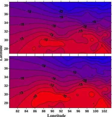
Second, the decreasing rate for latitude is greater in winter and smaller in summer and the decreasing rate for longitude is just the opposite indicating monthly mean surface air temperature distributed more parallel to latitude than to longitude in wintertime and more parallel to longitude than to latitude in summertime on the TP. As shown in Fig. 8, this feature has become less clear due to the decreasing rate for latitude becomes smaller and the decreasing rate for longitude becomes greater. Using our model to adjust all the station to same altitude (4800m), these features and changes of these features can be seen clearly as the calculated air temperature distributions on the TP as shown in Fig. 9 and Fig. 10. It is clear that warm area was shifted attitudinally in wintertime as show in
Fig.9 and were shifted longitudinally in summer as shown in Fig.
10. These mean that there was more warming in high latitude on the TP in wintertime and more warming in west part on the TP in summer.
82 84 86 88 90 92 94 96 98 100 102 28
30 32 34 36 38 28 30 32 34 36 38
Longitude
Latitude
Fig. 10 Distributions of air temperature adjusted by the linear model to 4800m in July (up: mean of 1956-1980; down: mean of 1981-2005)
E. Model application
As mentioned above, our linear model can be used not only to describe quantitatively the spatial distributions of surface air temperature but also to evaluate air temperature without observations using geographical information (latitude, longitude and altitude). However, due to that the model is deduced from the CMA data set and all the meteorological observatories on the TP are biased to the populated lower-elevation area (<4800m) in the eastern and southern TP and almost all of them are located in valleys or basin bottoms as shown in Fig. 1, the current conclusion may not be applicable for those high altitudes above 4800m ASL. It is not applicable, at lest for wintertime, to use the lapse rate to higher mountain slopes. Reference [9] has shown a greater lapse rate about 0.69ºC/100m between 4300m and 5500m ASL on a south slope of Mount Nyainqentanglha in the central part of the TP in July, which was affected by higher temperature between 4400m to 4800m, and a very lower lapse rate about 0.09ºC/100m at lower portion of slope (below 4800m) and a relatively larger lapse rate about 0.9ºC/100m at higher portion of the slope in wintertime due to an existence of temperature inversion in the valley.
Reference [10] has shown both observed air temperature at the meteorological observatory and estimated air temperature at the
overgrazed pasture at Damxung has increased about 2 degrees during past 47 years and this extreme air temperature increase is mainly caused by the land degradation due to overgrazing.
Therefore, long-term meteorological observation and the model modifications in high mountain region on the TP will be very important in high mountain regions in the future.
REFERENCES
[1] S. Kang, Y, Wu, Q. You, W. A. Flugel, N. Pepin and T. Yao, “Review of climate and cryospheric change in the Tibetan Plateau,”
Environmental research letters, 5 015101,
doi:10.1088/1748-9326/5/1/015101, 2010.
[2] X. Liu and B. Chen, “Climatic warming in the Tibetan Plateau during recent decades,” International Journal of Climatology. 20 (14), 1729–
1742, 2000.
[3] J. Qin, K. Yang. S. Liang, X. Guo, “The altitudinal dependence of recent rapid warming over the Tibetan Plateau,” Climatic Change, DOI 10.1007/s10584-009-9733-9, 2009.
[4] Q. You, S. Kang, N. Pepin and Y. Yan, “Relationship between trends in temperature extremes and elevation in the eastern and central Tibetan Plateau, 1961–2005,” Geophysical Research Letters, 35, L04704, doi:10.1029/2007GL032669d, 2008.
[5] D. Zheng, Q. “Zhang, Chapter 1 introduction,” in Mountain Genecology and Sustainable Development of the Tibetan Plateau. Kluwer Academic Publisihing, Dordrecht, pp. 1-17, 2000.
[6] O. W. Frauenfeld, T. Zhang, M. C. Serreze, “Climate change and variability using European Centre for Medium-Range Weather Forecasts reanalysis (ERA40) temperatures on the Tibetan Plateau,” Journal Geophysics Research, 110, D02101. doi:10.1029/2004JD005230, 2004.
[7] E. Kalnay, M. Cai, “Impact of urbanization and land-use change on climate,” Nature, 423 (6939), 528–531. 2003.
[8] M. Du, S. Kawashima, S. Yonemura, X. Zhang, S. Chen, “Mutual influence between human activities and climate change in the Tibetan Plateau during recent years,” Global Planet Change, 41, 241–249, 2004.
[9] M. Du, S. Kawashima, S. Yonemura, T. Yamada, X. Zhang, J. Liu, Y. Li, S. Gu and Y. Tang, “Temperature distribution in the high mountain regions on the Tibetan Plateau- Measurement and simulation”, in Proc.
MODSIM 2007 International Congress on Modelling and Simulation.
Modelling and Simulation Society of Australia and New Zealand, pp.
2146-2152. Available: http://www.mssanz.org.au/
[10] M. Du, S. Yonemura, X. Zhang, Y. He, J. Liu and S. Kawashima,
“Climatic Warming due to Overgrazing on the Tibetan Plateau – an Example at Damxung in the Central Part of the Tibetan Plateau,” Journal of Arid Land Studies, 22 (1), 119 -122. 2012.