Obstacle Detection Based on Occupancy Grid Maps Using Stereovision System

Obstacle Detection Based on Occupancy Grid Maps Using Stereovision System

著者 Kohara Kenji, Suganuma Naoki, Negishi Tatsuyuki, Nanri Takuya

journal or

publication title

International Journal of Intelligent Transportation Systems Research

volume 8

number 2

page range 85‑95

year 2010‑05‑01

URL http://hdl.handle.net/2297/23908

doi: 10.1007/s13177-010-0009-6

Obstacle Detection Based on Occupancy Grid Maps Using Stereovision System

Kenji Kohara

Naoki Suganuma

Tatsuyuki Negishi

Takuya Nanri

Graduate School of Natural Science & Technology, Kanazawa University

Institute of Science and Engineering, Kanazawa University

(Kakuma-cho, Kanazawa, Ishikawa 920-1192, JAPAN, +81-76-234-4714, [email protected], [email protected])

Tokyo R&D Center, Panasonic Corporation

(600 Saedo-cho, Tsuzuki-ku, Yokohama 224-8539, JAPAN, +81-50-3686-9034, {Negishi.tatsuyuki, nanri.takuya}@jp.panasonic.com)

We previously reported on an obstacle detection method using a stereovision system. The system generated disparity images that include three-dimensional spatial information. Using these images, obstacles could be detected, but some false positives were generated. In this paper, we attempt to eliminate this problem and propose a method that generates

Occupancy Grid Maps based on measurements from a stereovision system which leads to robust obstacle detection.

Furthermore, it is confirmed that high distance accuracy can be achieved by using our method.

Keywords: Stereovision System, Obstacle detection, Occupancy Grid Maps

1. Introduction

Recently, in order to tackle such problems as traffic accidents and traffic jams, much research has been carried out into the development of Intelligent Transport System (ITS). In the field of ITS research, driving support systems are among the most important research and development fields.

To realize a driving support system, it is necessary to recognize the surrounding environment. It is well known that stereovision systems are among the most practical approaches to this problem. For example, Sekiguchi et al.

[1] proposed a method to extract object information, such as preceding vehicles, lane markings, and guardrails, by using disparity images computed from individual images from two cameras. In this method, the objects are extracted by adopting some models to enhance the robustness. Broggi et al. [2], for the purpose of developing an autonomous vehicle, proposed a method to identify near and far obstacles by adaptively switching between three cameras. Kubota et al. [3] proposed a method to identify obstacles based on subtraction of geometrically transformed stereo images. This method has the advantage that the computational cost becomes low, because it is based on simple image subtraction.

However, almost all of these methods analyze the environment using a long baseline stereovision system.

For example, Sekiguchi et al. adopted a 350 mm baseline [1] and Broggi et al. used a baseline up to 1500 mm in length [2]. This is because a longer baseline improves the accuracy at larger distances. However, a system with an excessively long baseline introduces problems since it is difficult to be set up on a car, it is bletcherous, and it disturbs the driver’s view. On the other hand, obstacle

detection methods using a monocular camera have also been proposed. Franke et al. [4], for example, suggested a method to estimate distance based on relative image motion. However, there is a problem that the distance cannot be estimated unless the ego-vehicle moves for a while. Therefore, we developed and reported on a 120 mm baseline length stereovision system [5], [6]. This offers the advantage that it can be hidden behind the rear-view mirror in the vehicle. However, this system was found to have problems in that it produced some false positives while detecting obstacles. The characteristics of such false positives were that they appeared suddenly and rarely remained in the same position for long. Such problems are likely to affect not only our system but also systems that make use of raw sensor data. Moreover, our previous system suffered from a significant deterioration in distance accuracy as the baseline was shortened.

In this paper, we propose an obstacle detection method using Occupancy Grid Maps (OGM) [7] to solve these problems. In this method, the existence of an obstacle is represented as a posterior probability based on all past measurements obtained by the stereovision system from moment to moment. By using OGM, the number of false positives is reduced and obstacles can be robustly detected; moreover, the deterioration in distance accuracy that arises from baseline-shortening can be ameliorated.

2. Stereovision system

Figure 1(a) shows our experimental vehicle. The

stereovision system in the vehicle is mounted in front of

the rear-view mirror as shown in figure 1(b). The length

of the baseline is about 120 mm, so it is fairly unobtrusive and is almost hidden from the driver.

The stereovision system is a sensor that can measure distances from the vehicle to obstacles based on the principle of triangulation using two or more cameras. In this system, two cameras are installed parallel to each other. For a stereovision system with a baseline length of b, a focal length of f, and a principal point of (c

, c

), as shown in figure 2, the three-dimensional position of a target object P(X, Y, Z) determined from the disparity is given by







=

−

=

−

=

d bf Z

d c v b Y

d c u b X

v R

u R

/ / ) (

/ ) (

_(d=uL−uR)

(1),

where the subscripts L and R refer to the left and right cameras, respectively, and d is the disparity. Thus, we can obtain the three-dimensional position of a target object by computing the correspondence point between the right and left images. Figure 3 shows a disparity image where the magnitude of the disparity for each pixel is expressed with a gray scale value. In figure 3, it can be seen that there is a large amount of disparity even for textureless regions such as the road surface. This is

because, in this method, a LoG (Laplacian of Gaussian) filter [8] was adopted for image enhancement and this type of filter is well known to produce such effects. In our algorithm, obstacles are detected based on this disparity image.

3. Obstacle detection using virtual disparity image

In our previous reports [5], [6], we proposed an obstacle detection algorithm using a virtual disparity image (VDI). In this section, we briefly explain our obstacle detection method.

3.1. Road surface extraction

The v-disparity method [2], [9], [10] is generally used for road surface identification, owing to its simplicity and effectiveness. However, we previously reported that this method became inaccurate when the vehicle was moving fast on a curve.

In our previous reports [5], [6], we proposed the use of a virtual disparity image (VDI) to address this problem.

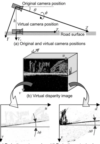
The VDI is a disparity image transformed to a virtual observation point as illustrated in figure 4(a). Figure 4(b) shows an example of a VDI.

Road surface h

θ

Y

Original camera position

Virtual camera position Y_v

φ

Z_v Z

(a) Original and virtual camera positions

(b) Virtual disparity image

(c) Projection onto u-vplane (d) Projection onto d-vplane

Figure 4. Road surface extraction from virtual

disparity image d

v

u

v

u

v

d

∆φ ∆θ

(a) Original image (b) Disparity image

Figure 3. Example of disparity image

Far (a) External view (b) Stereovision system

Figure 1. Experimental vehicle

P(X,Y,Z)

b

Y X

Z

f

v

Figure 2. Geometry of stereovision system

(c

, c

)

When using the VDI, the road surface can be extracted by projecting the VDI onto the d-v plane as in the traditional v-disparity approach. Additionally, we can also extract the road surface by projecting onto the u-v plane. Figures 4(c) and (d) show examples of projections of the VDI, and it can be seen that the road surface is clearly distinguishable in both planes. It is known that a flat plane in three-dimensional space also appears as a flat plane in disparity image space [9]. Therefore, in this case, the image projections in the d-v and u-v planes correspond to a “side view” and “front view” of three dimensional road scenes from the road surface viewpoint, respectively. Therefore, by extracting lines from both planes, we can estimate not only the height h and pitch angle θ from the d-v plane, but also the roll angle φ from the u-v plane. Further details concerning these algorithms are given in [5], [6].

3.2. Obstacle map generation

Next, we discuss an obstacle map generation method from the VDI. In the previous subsection, we described simple image projection onto the d-v and u-v planes from the virtual disparity image space. Here, we consider image projection onto the u-d plane from the virtual disparity image space.

The image projected onto the u-d plane contains information concerning obstacle maps, and the three-dimensional position of an obstacle can be estimated using this image. However, an image simply projected in this manner includes not only obstacles touching the road surface but also objects above the road, such as bridges, traffic signs, and signals. Therefore, in our method, only virtual disparity image space points satisfying H

are projected onto the u-d plane, where ∆H

is the height above the road surface, and H

and H

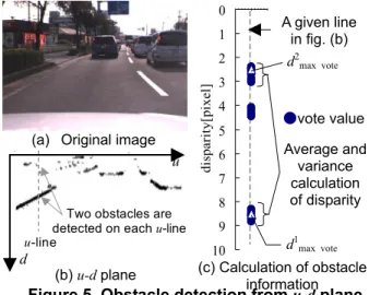
are predefined minimum and maximum heights above the road surface in real three-dimensional space. In our implementation, these values are set to –0.5 m and 2.5 m, respectively. Figure 5(b) shows an example of applying this type of projection to the image in figure 5(a).

We next explain the obstacle detection method using the u-d plane. Here, we consider the situation in which two different vehicles are present in front of the stereovision system, as shown in figure 6. In this situation, if a sensor such as a two-dimensional scanning laser range finder is used, only the near side object can be detected. However, a stereovision system can detect both objects if they exist in the image. Therefore, in our method, we take advantage of the stereovision: up to two objects are detected for each u-line (defined as a vertical line in the u-d plane, as shown in figure 5(b)).

Specifically, two disparities with maximum and semi-maximum vote values are detected on each u-line.

Here, the vote value means number of projected pixels from original disparity image in each pixel on projected image. Figure 5(c) shows disparity distribution along a

given line of figure 5(b). We define these disparities as d

(i = 1, 2). These positions are recorded as approximate obstacle positions. Moreover, pixels with disparities near these values in the VDI are searched for again based on these positions (u, d

). Finally, the average d

and variance σ

of these disparities are calculated by

2 2

2 i

u i

i i v u

i i i v u

N d d N d d

∑ −

=

=∑ σ

(2),

where d

is one of the detected disparities near d

and N

is number of such pixels. Subsequently, the d

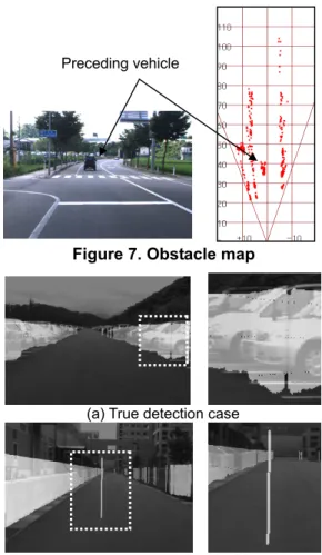
values obtained by equation (2) are adopted as obstacle positions on the u-line. Figure 7 illustrates an obstacle map in the vehicle coordinate system, calculated using this algorithm. In this figure, it can be seen that the distribution of points indicating preceding vehicles is spread out and distorted. As mentioned previously, this is most likely due to measurement errors resulting from the limited baseline length.

Figure 8 shows an original image superimposed raw obstacle detection data. Here, obstacles are highlighted from ground level up to a constant height based on the calculated obstacle distance.

In figure 8(a), the obstacles are detected accurately at their original positions. On the other hand, it can be seen

Figure 6. The case of two obstacles in front

dotted line rectangle is a background obstacle.

(a) Original image

d

u

u-line

Two obstacles are detected on each u-line

Figure 5. Obstacle detection from u-d plane

●vote value A given line

in fig. (b)

Average and variance calculation of disparity

(b) u-d plane (c) Calculation of obstacle information

d²max vote

0 1 2 3 4 5 6 7 8 9 10

disparity[pixel]

from figure 8(b) that there is a false positive in an area where no object exists on the road surface. This false positive is the result of noise that exists in the disparity image. Such noise tends to appear suddenly and in random positions. Therefore, in this paper, we propose a method to decrease the number of false positives using OGM [7] that can express the existence of obstacles as posterior probabilities based on all past measurements obtained by the stereovision from moment to moment.

4. Obstacle detection using Occupancy Grid Maps

In an OGM, the Cartesian coordinate space is partitioned into finitely many grid cells. For each cell, the posterior probability that an object exists is calculated based on all past measurements. Therefore, this algorithm can decrease the detection of false positives that appear suddenly.

In this section, we propose a method for the robust detection of obstacles using OGM.

4.1. Occupancy Grid Maps

As described above, in the OGM algorithm, the Cartesian coordinate space is partitioned into finitely

many grid cells. The posterior probability p(m

| z

, x

) of an obstacle being present is then calculated for each cell m

using information about the vehicle pose x

and measurements z

from the stereovision system. Here, x

represents the path of the vehicle defined by the sequence of all poses up to time t. Moreover, z

denotes the set of all measurements up to time t.

If we assume that the surrounding objects are static, p(m

| z

, x

) can be recursively calculated using a Binary Bayes Filter [11], where the log-odds l

are calculated, instead of p(m

| z

, x

), by

,1 0,

: 1 : 1 ,

: 1 : 1 ,

,

1 ( | , )

) ,

| log (

+ −

−

=



 





= −

ty x y x

t t y x

t t y t x

y x

l l Inv

x z m p

x z m

l p (3),

here













= −

) ,

| ( 1

) ,

| log (

, ,

t t y x

t t y x

x z m p

x z m

Inv p

(4),



 





= −

) ( 1

) log (

, 0 ,

,

y x y x y

x p m

m

l p

(5),

where p(m

| z

, x

) is a conditional probability given by the vehicle pose x

and a measurement z

on a grid cell m

at a time t. Inv denotes the inverse sensor model described in the next section. p(m

) is the prior probability that corresponds to the initial estimate before processing any sensor information.

The probabilities p(m

| z

, x

) can be easily recovered from the log-odds ratio l

:

) exp(

1 1 1 ) ,

| (

, :

1 : 1

, t

y x t

t y

x

z x l

m

p

(6).

Usually, in equation (3), p(m

) is set to 0.5 because the probability is unknown until measurements are taken.

Therefore l

is 0, and equation (3) is rewritten as follows:

l

Inv

l

(7).

Hereby l

can be continuously calculated as time passes. Moreover, the simple recursive addition improves the computation efficiency.

4.2. Inverse sensor model

The inverse sensor model allows us to express the probabilities in all grid cells based on the measurements z

. In this paper, this model is built on each u*-line in the u-d plane, and p(m

| z

, x

) is calculated based on

*)

*,

1 (u d

p_Occ

,

and

as shown in figure 9 and by following equation:

*)]

*, (

*),

*, (

*),

*, ( max[

) ,

| (

2 1

,

d u p d u p d u p

x z m p

Free Occ

Occ t t y x

=

(8),

where (u*, d*) denotes the u-d plane coordinate of each grid cell m

transformed from the vehicle coordinates by using equation (1). Actually, u* is not an integer, but, in our implementation, rounded values are used instead of

(b) False positive case

Figure 8. Obstacle detection results using raw data Figure 7. Obstacle map

Preceding vehicle

Figure 9. Inverse sensor model

max , Occ2 max

p

, 1Occ

p

0.5 p

− 1

d Near d

d

Far

1Occ

p

p(m

| z

x

) p

1.0

Occ2

p

p

the original u*.

We detail the particulars in the next subsection.

4.2.1. Probability based on measurementp_Occⁱ (u*,d*).

We now assume that objects are observed by the stereovision system at positions d

(i = 1, 2) given by equation (2) on the u*-line in the u-d plane. At this time, because the d

values contain measuring errors, it is necessary to assign probabilities based on variances. We define these probabilities as p

( u *, d *) calculated by







 −

−

⋅

= ^,max ₂^{*, 2}

2 )

* exp (

*)

*, (

*)

*, (

i i

t u i

Occ i

Error

d d d

u p d u

p σ

(9),

where σ

is the variance of d

obtained by equation (2), and p

( u *, d *) is a parameter representing the maximum probability as explained in the next subsection.

In the area beyond the position d

, however, the existence of objects is unknown since they can not be observed. We define the probability in this unobservable area as p

(u*, d*) calculated by





≤

= >

)

* ( 5 . 0

)

* ( 0 .

*) 0

*, (

*,

*, i

t u

i t u

Unk d d

d d d

u

p 　　

(10).

Finally, the probabilities

based on measurements are calculated by

*)]

*, (

*),

*, ( max[

*)

*,

(u d p u d p u d

pⁱ_Occ = _Unk ⁱ_Error

(11).

4.2.2. Probability based on road surface appearance

*)

*, (u d

p_Free and p_Occ^i,max(u*,d*).

On the other hand, objects may exist in the area between the vehicle position and the measurement point d

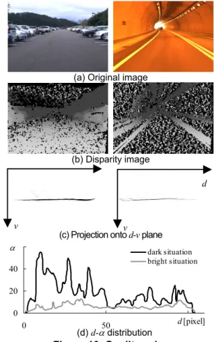
. Figure 10(a) shows original images under bright (left) and dark (right) conditions. Figure 10(b) shows the corresponding disparity images.

As shown in figure 10(b), the disparity image in the dark tunnel is the noisier of the two since the original image was noisy. Therefore, in some situations it cannot be determined whether objects exist or not because of difficulties analyzing the disparity image. In such cases, it is necessary to assign a reasonable probability in the OGM. We define this probability as p

(u*, d*).

Figure 10(c) shows projection images onto the d-v

plane based on the disparity image in each situation;

these images represent the appearance of the road surface in the disparity images. In these images, the lighter the contrast, the less the road surface appears. Therefore, from figure 10(c), the road surface appearance in the tunnel is less than in bright situations. In other words, in dark situations, disparities are difficult to calculate.

Therefore we proposed a method of adaptively calculating p

(u*, d*) based on road surface appearances.

Specifically, we calculate the road surface appearance [12] by analyzing two images projected onto the d-v and u-v planes, and we define the evaluated values as α(d*) and α(u*), respectively. For each vertical line in each image, these values are calculated by

*) ( /

*) (

*)

(d σ² d Nd

α =

(12),

*) ( /

*) (

*)

(u σ² u N u

α =

(13),

where

(d*) and σ

(u*) are the variances of the vote values of the disparities near the road surface position in the d-v and u-v plane, respectively. N(d*) and N(u*) are the total vote values of the disparities in the considered areas. In equation (12), if σ

(d*) is large, the road surface position is ambiguous because

large. By the same token, if N(d*) is small, observed road surface appearances become scarce. Therefore, the larger

v

(a) Original image

(b) Disparity image

(c) Projection onto d-v plane

(d) d-α distribution

Figure 10. Quality value α

Right-side images: dark conditions.

d

v

0 20 40 60

0 50 100

dark situation bright situation

d[pixel]

α

appearances are. Figure 10(d) shows α(d*) in bright and dark situations, and it is seen to be larger in the dark situation.

Moreover, by multiplying α(d*) by α(u*), the road surface appearance at the coordinates (u*, d*) in the u-d plane is evaluated. We define this value as α(u*, d*) and calculate it by

*) (

*) (

*)

*,

(u d α u α d

α = ･

(14).

In our algorithm, we adopt this value as p

(u*, d*) after normalizing it to a value between 0 and 0.5. It is limited to an upper value of 0.5 because p

(u*, d*) is the probability to express that objects don’t exist.

On the other hand,

, which represents the maximum value in the probability distribution, also depends on the road surface appearance because measurements contain much more noise in dark situations than in bright ones. Therefore, it is necessary that the higher p

(u*, d*) is, the lower

becomes, and the OGM can be robustly generated even in such noisy situations. This probability

is calculated by

*)]

*, ( 0 . 1 , 6 . 0 max[

*)

*,

max(

, u d p u d

p_Occⁱ = 　 − _Free

(15),

where the reason we set the minimum value to 0.6 is to influence measurements in the OGM even when p

(u*, d*) becomes 0.5 due to the scarce appearance of the road surface. In other words, if the minimum value were set to 0.5, the OGM would rarely represent obstacle maps even if the measurements were accurate.

As stated above, the OGM can be updated by applying a Binary Bayes Filter and inverse sensor model, and we proposed a method for the inverse sensor model that uses not only measurements but also the road surface appearance to robustly generate the OGM.

4.3. Vehicle pose estimation using scan matching In the previous section, the OGM was generated based on the assumption that the vehicle pose is known.

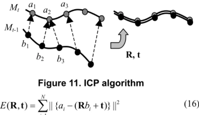
Therefore, in order to build a consistent map of the environment, good vehicle localization is required. The problem of simultaneously estimating vehicle pose and a consistency map is called Simultaneous Localization and Mapping (SLAM). The SLAM problem can be solved by a scan matching algorithm [13], [14], and an Iterative Closest Point (ICP) algorithm [15] is adopted in our implementation.

The ICP algorithm can calculate the coordinate transformation parameters that minimize the error between the two obstacle maps by iterative calculations.

Figure 11 shows an example of this method. We assume two obstacle maps M

and M

exist as shown in figure 11. Here, M

is a map at time t-1 and M

is a map at time t, and a

and b

correspond to the elements of these maps, respectively. Then, the minimum distance between each point in M

and M

is calculated, and the sum of the squares of these distances is calculated by

2 1

||

} ) ( {

||

) ,

( ∑

=

+

−

= ^N

i

i

i

b

a

E

(16),

where N is number of minimum-distance combinations,

error E relates to the distance between M

and M

. The map M

is then repeatedly transformed until E is minimized, which results in an estimation of R and t.

In our implementation, we use the steepest descent method to calculate the optimal solutions for R and t in equation (16), and the initial values of R and t are taken from the vehicle pose estimated using velocity and yaw rate sensors.

Finally, an accurate vehicle pose x

is updated by using both the R and t values obtained by the ICP algorithm.

5. Experiment

In the previous section, the method of obstacle detection using the OGM was described. In this chapter, we present the results of obstacle detection using the OGM and estimate its validity; in addition we compare the distance accuracy between the raw data and OGM.

5.1. Evaluation of obstacle detection using OGM First, the results of obstacle detection using the proposed method (OGM) are compared with the those using the conventional method (raw data). In this experiment, the detected obstacle positions are displayed in the original image by superimposing the raw data and the OGM as shown in figure 12(a) and (b). In the OGM, the high probability regions are displayed on the original image. The grid cell size in the OGM is 0.2 m × 0.2 m and the map region is 40 m × 120 m. Moreover, in the OGM, the darker the grid cell is, the higher the probability is. Mid-tone areas represent probabilities of about 0.5, where it is unknown whether an obstacle exists or not.

It can be seen from figure 12(a) that there are some false positives in front of the vehicle. On the other hand, these do not appear in figure 12(b). This is because the data points corresponding to these false positives appear suddenly in the low probability region of the OGM, as shown in figure 12(c). Accordingly, by calculating the probability from moment to moment, sudden false positives can be eliminated. Furthermore, by accumulating obstacle maps through time, it can be seen that the highlighted regions corresponding to obstacles in

M

M

b

b

b

a

a

a

R, t

Figure 11. ICP algorithm

figure 12(b) are denser than the raw data in figure 12(a), in particular in the far left-side region.

Figure 13 illustrates the results of obstacle detection while driving in a tunnel. As previously mentioned, a large amount of noise appears in the disparity images in such dark situations. Thus, in figure 13(a), which displays the raw data, many false positives appear on a lane marking. However, this does not occur in figure 13(b), which displays the OGM. This is again because the measurement data that correspond to them exist in the low probability area of the OGM. Thus, it can be seen that obstacles can be detected robustly using the proposed method.

Moreover, we performed tests to evaluate the robustness of the method against false positive. In this experiment, 200 frames were examined. In the worst frame, there were 370 measurements calculated by equation (2) in the frame, and 7 of them (1.9%) were false positives. However, the proposed method completely eliminated these false positives.

5.2. Evaluation of OGM validity

In section 4.2, we described the inverse sensor model based on road surface appearance to handle situations were very few disparities occurred. In this section, we evaluate the effectiveness of this model in generating the OGM in such situations.

Specifically, we evaluate how the probability p

that indicates the road surface appearance as shown in equation (14) affects obstacle detection and the OGM.

Figure 14 depicts obstacle detection results in a tunnel using the OGM method. Figure 14 (a) shows the case for using our model but excluding p

, and (b) shows the case when p

is included. Moreover, (c) and (d) show the OGMs corresponding to (a) and (b), respectively.

In figure 14, there is little difference between the obstacle detection results shown in (a) and (b). However, in figure 14(c), the OGM indicates a low probability that no obstacle exists even in regions further than the physical tunnel wall. On the other hand, in figure 14(d), it can be seen that the OGM correctly assesses that such area is unknown whether an obstacle exists or not.

Therefore, we can conclude that the use of p

can reduce inaccurate estimations in the OGM.

5.3. Evaluation of distance accuracy

Next, we evaluate the distance accuracy of the OGM.

Here, the distance accuracy calculated by OGM is compared with that determined from the raw data using a stereovision system whose baseline length is 120 mm.

Additionally, a comparison is made with the raw data from a 350 mm baseline system.

In this experiment, distance accuracy is evaluated by fixed-point observation of obstacles that are placed at 10 m intervals from the stereovision system up to a distance of 100 m, as shown in figure 15. Figure 16 depicts examples of obstacle maps that the preceding vehicle is

by raw data

(b) Extracted obstacles with OGM (c) OGM

Figure 12. Comparison of obstacle detection

Figure 13. Comparison of obstacle detection in tunnel

(c) OGM (a) Extracted obstacles

with raw data

(b) Extracted obstacles with OGM

(a) Extracted obstacles by OGM without pfree

(b) Extracted obstacles by OGM with pfree

(c) OGM

without p_free (d) OGM with p_free

Figure 14. Comparison of OGM in a tunnel

with and without p

placed at 60 m generated by the three systems. In figure 16(c), the obstacle positions are calculated by extracting grid cells that have peak probability on an OGM. In this figure, the measurements for 120 mm system seems to have large measurement error compared with those for 350 mm system. On the other hand, by using OGM, it is find from figure 16(c) that the measurement error is obviously reduced.

Figure 17 shows the standard deviation results for the three systems. In this figure, the standard deviations of these measurements over 15 frames (1 second) are calculated at each position. It can be seen that the results for the 120 mm system (without OGM) are considerable worse than those for the 350 mm system, particularly at large distances. This is because the longer the baseline is, the higher the disparity accuracy becomes. However, for the 120 mm system with OGM, the standard deviations are much lower than those for the same baseline length without OGM. For example, for a distance of 100 m,

OGM improves the accuracy by approximately 5 times.

Moreover, the 120 mm system with OGM outperforms even the 350 mm system at distances of 40 m or above.

Thus, even if we use a short baseline stereovision system, high distance accuracy better than a system with 3 times the baseline length can be achieved.

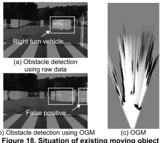
However, some problematic situations still exist.

Figure 18 illustrates the results of obstacle detection in the situation where moving objects exist. To generate the OGM, as noted in the section 4.1, it is required that the surrounding objects are static. In this situation, a part of intersection that is actually clear of traffic originally seems to be blocked by a moving vehicle for a period of time. This is because the data corresponding to this vehicle do not appear in the same position because this vehicle moves.

Actually, the false positive clears up over time because the probability in the false positive region becomes low if nothing is observed in this area after the vehicle moves away.

Nevertheless, one method of approaching this problem may be to discard older maps from memory. Additionally, a method of detecting and tracking moving objects so that they do not influence the OGM may be effective.

Currently, we are studying the latter approach based on the fact that a moving object does not appear in the same position every moment.

6. Conclusion

In this paper, we proposed an obstacle detection method using OGM to overcome some problems caused by shortening the baseline of stereovision systems. Our method is summarized as follows:

・

By using OGM, false positives in the conventional method could be eliminated and dense obstacle maps could be generated.

・

In the OGM algorithm, an inverse sensor model considering road surface appearance was proposed.

(c) OGM

Figure 18. Situation of existing moving object

(a) Obstacle detection using raw data

(b) Obstacle detection using OGM Right turn vehicle

False positive

Figure 15. Situation of fixed-point observation

(a) 120 mm (b) 350 mm (c) 120 mm with OGM

Figure.16. Example of obstacle maps at 60 m

0 1 2 3 4 5 6

0 50 100

Distance to target [m]

Standard deviation [m]

120mm 350mm

120mm with OGM

Figure 17. Comparison of standard deviation of

distance accuracy at each position

By using this model, consistent OGM which took into account the quality of disparity images could be generated.

・

The reduction in stereovision accuracy caused by shortening the baseline was improved using the proposed method, and it was confirmed that the distance accuracy during obstacle detection was the same or better than a system with a baseline triple the length.

In view of these results, it can be concluded that obstacle detection using OGM is an effective method in various situations, even when a large amount of sensor noise exists, and it can be easily applied to other sensing methods such as laser range finders.

7. References

[1] H.Sekiguchi, et.al, “Development of Driving Assist System by New Stereo Camera”, SUBARU Technical review, vol.35, pp.109-119, 2008

[2] A.Broggi, C.Caraffi, P.P.Porta, P.Zani, “The Single Frame Stereo Vision System for Reliable Obstacle Detection used during the 2005 DARPA Grand Challenge on TerraMax”, Proc.

of the 2006 IEEE Intelligent Transportation Systems Conference (ITSC2006), pp.745- 752, 2006

[3] S.Kubota, T.Nakano, Y.Okamoto, “A Global Optimization Algorithm for Real-Time On-Board Stereo Obstacle Detection Systems”, Proceedings of the IEEE Intelligent Vehicle Symposium, pp.7-12, 2007

[4] U.Franke, C.Rabe, “Kalman Filter based depth from motion with fast convergence”, Proceedings of the IEEE Intelligent Vehicle Symposium, pp.180-185, 2005

[5] M.Shimoyama, N.Suganuma, T.Sota, T.Nanri, “An obstacle extraction method using virtual disparity image -Stabilization of road surface estimation using Kalman Filter-”，Proceedings of 6th ITS Symposium 2007，pp.337-342, 2007

[6] N.Suganuma, N.Fujiwara, “An Obstacle Extraction Method Using Virtual Disparity Image”，Proc. of the 2007 IEEE Intelligent Vehicles Symposium，pp.456-461，2007 [7] A.Elfes Occupancy grids: a probabilistic framework for robot perception and navigation. PhD thesis, Carnegie Mellon University, 1989

[8] T.Noguchi, S.Kimura, “Data Compression of LoG Filter Output for Pre-Processing in StereoMatching”, Institute of Electronics, Information, and Communication Engineers, vol.

J83-D-II No.9, pp.1952-1956, 2000

[9] N.Suganuma, N.Fujiwara, K.Senda，“Vehicle Front Environment Recognition Using Stereo Vision”， Transactions of the Japan Society of Mechanical Engineers, Series (C), Vol.71, No.703，pp881-887，2005

[10] N.Soquet, D.Aubert, N.Hautiere, “Road Segmentation

Supervised by an Extended V-Disparity Algorithm for Autonomous Navigation”, Proc. of the 2007 IEEE Intelligent Vehicles Symposium (IV2007), pp.456-461, 2007

[11] S.Thrun, W.Burgard, D.Fox, “Probabilistic Robotics”, MIT Press, Cambridge, Massachusetts, pp.94-96

[12] N.Suganuma, M.Shimoyama, N.Fujiwara, “Obstacle Detection Using Virtual Disparity Image for Non-Flat Road”, Proc. of the 2008 IEEE Intelligent Vehicles Symposium, pp.596~601, 2008

[13] Dissanayake, G., Paxman, J.P., Valls Miro, J., Thane, Oliver & Tuan Thi, Hue. “Robotics for urban search and rescue”, In Proceedings of the IEEE First International Conference on Industrial and Information Systems (ICIIS 2006), pp. 294-298, 2006

[14] T. D. Vu, O. Aycard, N. Appenrodt, “Online Localization and Mapping with Moving Object Tracking in Dynamic Outdoor Environments”, Proc. of the 2007 IEEE Intelligent Vehicles Symposium, pp.190~195, 2007

[15] F. Lu and E. Milios, “Globally Consistent Range Scan Alignment for Environment Mapping”, Autonomous Robots 4 (April)(1997), pp. 333-349, 1997

Kenji Kohara is a Master course student of Natural Science and Technology, Kanazawa University. He received a B.E.

degree from Kanazawa University in 2008.

His research interests include visual assistance for drivers and image processing.

Naoki Suganuma is Lecturer of Kanazawa University. He received a Doctor of Engineering degree from Kanazawa University in 2002. His major research interests are environment perception and control of unmanned autonomous vehicles.

He is a member of JSME, SICE, RSJ and JSAE.

Negishi Tatsuyuki is a team leader at Panasonic Corporation. He received a Master of Engineering degree from Tokyo Institute of Technology in 1995. His research interest is image processing.

Takuya Nanri is an engineer at Panasonic Corporation. He received a Masters degree in Information Science and Technology from Tokyo University in 2006. His research interests are computer vision and pattern recognition.