Improving performance of deadbeat servomechanism by means of multirate input control ¶ §

ISSN 1344-8803, CSSE-14 April 6, 2001

Improving performance of deadbeat servomechanism by means of multirate input control ^{¶ §}

Hiroshi Ito ^†‡

† Department of Control Engineering and Science, Kyushu Institute of Technology 680-4 Kawazu, Iizuka, Fukuoka 820-8502, Japan

Phone: (+81)948-29-7717, Fax: (+81)948-29-7709 E-mail: [email protected]

Abstract: In this paper, an state-space approach to deadbeat servomechanism design is proposed using multirate input control. This paper focuses advantage of multirate control over conventional single-rate control. To achieve settling time specified, multirate controllers require less frequent sampling of measurement than single-rate ones. Multirate input mechanism can yield shorter settling time than single-rate control using the same frequency of sampling. However, multirate control often exhibits intersample ripple. Nevertheless, this paper demonstrates that the undesir- able effect of multirate input on the steady-state response can be removed completely to accomplish ripple-free deadbeat, keeping the settling time short using multirate mechanism at the same time.

Furthermore, the paper proposes a design method for multirate ripple-free deadbeat control which guarantees robustness against continuous-time model uncertainty and disturbance.

Keywords: deadbeat tracking, ripple-free servomechanism, multirate sampled-data control, ro- bustness, parametrization, continuous-time measure

¶

Technical Report in Computer Science and Systems Engineering, Log Number CSSE-14, ISSN 1344-8803. c 2001 Kyushu Institute of Technology

§

The current version of the paper was completed by August 12, 1999. Its shortened version was presented at 2000 American Control Conference, pp.169-174, Chicago, USA, June 28, 2000. A brief version was also presented at The 22nd SICE Symposium on Dynamical System Theory, pp.351-356, Utsunomia, Japan, October 28, 1999.

‡

Author for correspondence

1 Introduction

In modern control technology, there has been a growing demand for multirate digital control to seek better performance[15, 13]. Multirate control is suitable for systems having widely different time constants. Multiple rates also naturally arise from practical hardware limitations such as allowable rates of sampling and hold mechanisms in actuators, sensors and processors. In some situations, mulirate control has been found to be superior to single-rate control. For example, simultaneous stabilization, pole assignment and strong stabi- lization can be reduced to comparatively easy problems by introducing multirate input or generalized hold functions[3, 14, 23]. The mechanism can relocate zeros[27]. A comprehensive list of abilities of multirate con- trol is available in [2]. Although multi-rate possesses seemingly desirable features, advantage over single-rate control is a matter of debate. For control scheme having different sampling and hold periods one another, comparison of their performance is delicate. For instance, contribution of discrete zeros and poles, discrete frequency response and discrete norm to systems behavior is not uniform since performance measures are not based on the same time variable. Several people have pointed out that use of multirate control may result in sensitivity and robustness difficulties[27, 7, 9]. Control signal may become highly irregular and control can exhibit unacceptable intersample ripple[4]. Although performance of a multirate system is good in discrete time, the performance can be seriously bad in continuous time at the same time. Clearly, intersample behavior and continuous-time based measure are keys to a fair evaluation of performance and robustness. Capabilities and limitations of multirate control depends on objectives. This paper does not include a long list of previous contributions. Limitations and advantages of multirate control are explained rigorously in [2].

Deadbeat control is one of control problems which are not included in the survey [2]. This paper explores the capability issue of multirate control though deadbeat servomechanism. To the best of the author’s knowl- edge, the issue of comparison between multirate and single-rate has not been discussed deeply yet in the literature of deadbeat control. Deadbeat control has been studied for more than four decades[5, 24, 22, 32].

Since single-rate deadbeat design sometimes results in serious ripple between sampling instants especially in input-output or frequency domain approaches, ripple-free servomechanism has attracted much attention[8, 30, 28, 33, 12]. As for multirate design, several methods are available to cope with situations where periods of sampling and hold are determined a priori by hardware or time scales of the plant[11]. Little is known about how to exploit multiple periods for achieving better performance[2] in comparison to single-rate control.

This paper addresses the design problem of deadbeat state-feedback control by exploiting multirate input mechanism. The system output is required to track a step reference signal with zero steady-state error in finite time from any initial state. In contrast with previous studies typically in frequency domain, this paper allows the initial state to be arbitrary. A state-space approach is developed for deadbeat, ripple-free deadbeat and robust ripple-free deadbeat problems. Instead of looking at ‘the number of steps’ for settling, settling

‘time’ is employed to compare performance of multirate and single-rate control fairly. This paper first shows that multirate input control can be superior to single-rate control in the deadbeat problem. Then, this paper describes that the multirate mechanism sometimes exhibits oscillatory behavior of the manipulating input and that causes intersample ripple. This contrasts with the fact that single-rate state-feedback design though the state-space approach always results in ripple-free deadbeat. This paper shows how to remove the negative effect of multirate input on the steady-state response, while the multirate system retains quick transient response. Thereby, multirate control can be still better than single-rate control, taking account of ripple.

Finally, the paper develops a method of robustifying the ripple-free multirate control against continuous-time

z ⁻¹ K Hold L

Plant - - - - - - -

6 6

-

6

a a a a

g g q g q

y r [ k ] e [ k ] z [ k ] q [ i ]

p [ i ]

u [ i ] u ( t )

x [ k ]

x ( t ) y ( t ) y [ k ]

N T T

−

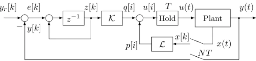
Figure 1: Multirate control for deadbeat servomechanism

model uncertainty and continuous-time disturbances. A parametrization of ripple-free deadbeat multirate controllers having specified settling time is given and an optimization problem for solving the robustness problem is formulated. All proofs are collected in Appendix.

2 Deadbeat servomechanism

2.1 Deadbeat tracking using multirate input

Consider an SISO continuous-time linear time-invariant system described by x ˙ ( t ) = A c x ( t ) + B c u ( t ) , x ( t ) ∈ R ⁿ

y ( t ) = C c x ( t ) (1)

The initial time is t = 0. The plant (1) is supposed to satisfy the following standard assumptions.

Assumption 1 The triplet ( A c , B c , C c ) is controllable and observable.

Assumption 2 The continuous-time system (1) does not have zeros at the origin.

This paper focuses on the multirate input mechanism as follows:

x [ k ] = x ( kN T ) , y [ k ] = y ( kN T ) , k = 0 , 1 , 2 , . . . (2) u ( t ) = u [ i ] , iT ≤ t ≤ ( i + 1) T, i = 0 , 1 , 2 , . . . (3) where the sampling period for x ( t ) and y ( t ) is N T and the period of zero-order hold for u ( t ) is T > 0. The positive integer N is called the input multiplicity. The control objective is to design multirate input control which makes the output signal y to track a step reference y r with zero steady-state error in finite time. The paper considers the state feedback configuration shown in figure 1 which has a discrete-time internal model with period N T in the feedback loop. x The mappings L, K are linear operators satisfying

L : {x [ k ] } → {p [ kN ] , · · ·, p [( k + 1) N − 1] } (4)

K : {z [ k ] } → {q [ kN ] , · · ·, q [( k + 1) N − 1] } (5)

u [ i ] = p [ i ] + q [ i ] , k, i = 0 , 1 , 2 , . . . (6)

which are time-invariant and static. In other words, there exist real row vectors L j , K j such that

p [ kN + j − 1] = L j x [ k ] , j = 1 , 2 , . . ., N (7)

q [ kN + j − 1] = K j z [ k ] (8)

hold. Let y r ( t ) be a unit step signal and y r [ k ] denotes the discrete counterpart. The state variable of the discrete internal model is denoted by z [ k ]. The deadbeat problem is stated formally as follows:

Find L j and K j , j = 1 , . . . , N with which the system shown in figure 1 is internally stable and y [ k ] satisfies y [ k ] = y r [ k ] , ∀k ≥ τ, ∀x (0) ∈ R ⁿ , ∀z [0] ∈ R (9) for a finite integer τ ≥ 0.

The minimum integer τ satisfying (9) for all initial values x (0), z [0] is called the settling steps, which is denoted by τ d . The real number τ c = τ d N T is called the settling time. This paper attaches importance to the settling time rather than the settling steps. We can compare performance of single-rate design and multirate design fairly using the settling time.

2.2 Design of multirate feedback gain

Let ˆ u [ k ] be defined by

u ˆ [ k ] =



 

 

u [( k + 1) N − 1]

.. . u [ kN + 1]

u [ kN ]



 

  (10)

which is the discrete-time lifted signal of u [ k ] [26, 29]．Then, the plant (1) can be represented as x [ k + 1] = A ^N x [ k ] + ˆ B u ˆ [ k ]

y [ k ] = ˆ Cx [ k ] (11)

A = e ^A

^T , B = _T

0 e ^A

^τ dτ B c , C ˆ = C c

B ˆ =

B AB · · · A ^{N −1} B = B ˆ 1 , · · ·, B ˆ N

This system (11) is called the ‘lifted’ plant. If the triplet ( A c , B c , C c ) is controllable and observable, ( A ^N , B, ˆ C ˆ ) is also controllable and observable for almost all T > 0 [20]. Thus, we reasonably replace Assumption 1 by the following.

Assumption 1’ The triplet ( A ^N , B, ˆ C ˆ ) is controllable and observable.

By using discrete signals of period N T , the closed-loop system in figure 1 is described as x ˜ [ k + 1] = ˜ A x ˜ [ k ] + ˜ B u ˆ [ k ] + ˜ d

y [ k ] = ˜ C x ˜ [ k ] , u ˆ [ k ] = −F x ˜ [ k ] (12) x ˜ [ k ] =

x [ k ] z [ k ]

, d ˜ =

0 y r

A ˜ =

A ^N 0

− C ˆ 1

, B ˜ = B ˆ

0

= B ˜ 1 , · · ·, B ˜ N

C ˜ = C ˆ 0 , F =

L K

where L and K are lifted representations of L and K , respectively.

L =



  L 1

.. . L N



  , K =



  K 1

.. . K N



  (13)

This paper refers to F as the multirate feedback gain. Internal stability of the discrete-time system (12) is equivalent to the internal stability of the multirate sampled-data system in figure 1 [20]. This equivalence and the next lemma allow us to exploit the representation (12) for the deadbeat design.

Lemma 1 For any complex number z , ( A ^N , B, ˆ C ˆ ) satisfies rank

zI − A ^N 0 B ˆ C ˆ z − 1 0

= n + 1 (14)

The pair ( ˜ A, B ˜ ) is controllable regardless of N . Let n max denote the controllability index of ( ˜ A, B ˜ ).

n max = max {n ₁ , n 2 , · · ·, n N } n i = min

j : ˜ A ^j B ˜ i ∈ span

B, ˜ A ˜ B, ˜ · · ·, A ˜ ^j−1 B, ˜ A ˜ ^j B ˜ 1 , · · · , A ˜ ^j B ˜ i−1

Due to Lemma 1, we have

s N = n + 1 , s r = r i=1

n i , r = 1 , 2 , . . ., N

Theorem 1 Given an arbitrarily integer N > 0, there exists a multirate feedback gain F which solves the deadbeat problem with τ d = n max . Furthermore, the settling discrete time of x ˜ [ k ] cannot be less than n max . Proof of the theorem employs the theory of deadbeat control for MIMO discrete-time systems. Due to Lemma 1, there exists a non-singular matrix S which transforms ( ˜ A, B ˜ ) into the controllable canonical form ( A s , B s ), which are consistent with

A s = S AS ˜ ⁻¹ , B s = S B ˜ (15)

A s =



 

 

 

 

 

U ¯ 1 0 · · · 0 a 1

0 U ¯ 2 · · · 0 a 2

.. . .. . . . . .. . 0 0 · · · U ¯ N

a N



 

 

 

 

 

, a i ∈ R ^1×(n+1) i = 1 , 2 , . . ., N

B s =



 

 

 

 

 

0

1 b 12 · · · b 1N

0

0 1 b 23 · · · .. .

0 0 · · · 0 1



 

 

 

 

 

=



 

 

 

 

  0 b 1

0 b 2

.. . 0 b N



 

 

 

 

 

∈ R ^(n+1)×N

U ¯ i =



 

 



0 1 0

0 0 1 . . . . .. ...

0 1



 

 

 ∈ R ⁽ⁿ

^−1)×n

Let the feedback gain F be chosen as

F = GF s S, G =



 

  b 1

b 2

.. . b N



 

 

−1

, F s =



 

  a 1

a 2

.. . a N



 

  (16)

Then, we have

( A s − B s GF s ) ⁱ = 0 , ∀i ≥ n max (17)

Due to the discrete-time internal model, the closed-loop system has the property C ˆ 0 =

0 1 ( I − A ˜ + ˜ BF ) This equation implies that y [ k ] fulfills the tracking requirement

y [ ∞ ] = y r

regardless of precise values of A c , B c , C c , F whenever the closed-loop system is internally stable.

2.3 Settling time for deadbeat

We shall examine the setting time of the deadbeat servomechanism proposed by the multirate feedback gain (16). From Theorem 1, settling time is n max N T . The smaller n max N is, the shorter settling time the system has. Since rank ˜ B < n + 1 holds obviously for all N , n max = 1 cannot be fulfilled. To examine the possibility of achieving n max = 2, we focus on the matrix

V = B ˜ A ˜ B ˜ (18)

The size of V is ( n + 1) × 2 N . The matrix has full-row rank only if N ≥ ( n + 1) / 2 for n : odd

N ≥ ( n + 2) / 2 for n : even (19)

By assumption, ( ˜ A, B ˜ ) is controllable for any N . Taking the smallest N in (19), we obtain the following.

Theorem 2 There always exists a multirate feedback gain F solving the deadbeat problem and (i) the settling time is ( n + 1) T if n is odd.

(ii) the settling time is ( n + 2) T if n is even.

Such a multirate feedback gain is obtained from F = GF s S together with (15) and (16), taking N = ( n + 1) / 2 for odd n , or N = ( n + 2) / 2 for even n . Since the single-rate case N = 1 implies n max = n + 1 and n max N = n + 1, the following fact is straightforward from Theorem 2.

Corollary 1 The deadbeat problem can be solved by either of multirate control and single-rate control. Fur- thermore, there exists a multirate controller which requires less number of sampling for accomplishing deadbeat than single-rate controllers, and

(i) settling time is the same as that of single-rate when n is odd.

(ii) settling time is longer than that of single-rate by only T when n is even.

3 Ripple-free deadbeat servomechanism

3.1 Design of ripple-free feedback gain

The method proposed in the previous section often allows the deadbeat response to have ripple between sampling instants. The existence of ripple in a multirate control system is characterized by the continuous- time behavior of control input.

Theorem 3 Suppose that a multirate control system posses deadbeat tracking response at sampling instants for step input. The response does not exhibit ripple between sampling instants if and only if the steady-state input u ( t ) takes a constant value.

In the single-rate case, continuous-time signal u ( t ) takes a constant value if and only if the discrete signal u [ k ](= ˆ u [ k ]) with the period N T of sampler is constant. The steady-state u [ k ] =constant is necessary and sufficient for ripple-free deadbeat tracking[28, 8, 25]. Thus, Theorem 3 is nothing but a natural extension of this fact to the multirate input case. Consider again the control law given by (16). The steady-state of discrete time signal u [ i ] is obtained from the lifted signal

u ˆ s = −F x ˜ [ ∞ ] = −F ( I − A ˜ + ˜ BF ) ⁻¹ d ˜ (20) which is the steady-state of ˆ u [ k ]. It is obvious that the input u ( t ) becomes constant after completion of deadbeat in the single-rate case. However, this is not the case for multirate control N > 1. Although the steady-state u ( t ) repeats the same profile with period N T , the signal is unnecessarily constant all times. Too see this point, let a matrix J be defined by

J =



 

 



1 − 1 0 · · · 0 0 1 . .. ... .. . .. . . . . . . . − 1 0 0 · · · 0 1 − 1



 

 

 (21)

The feedback gain F proposed in the previous section yields a constant steady-state input if and only if

JGF s ( I + A s − B s GF s ) S



 

  0

.. . 0 1



 

  = 0 (22)

holds. In the process of obtaining (22), the properties ( I − A ˜ + ˜ BF ) ⁻¹ =

∞ i=0

( ˜ A − BF ˜ ) ⁱ

( ˜ A − BF ˜ ) ² = 0 (23)

are applied to (20). The condition (22) relies directly only on the plant data ( A c , B c , C c ) so that ripple usually

remains after deadbeat settling. The multirate control is the very technique which allows input signal to take

multiple values in one frame period N T in order to manage to achieve the design objective. In some situations,

it may cause undesirable oscillation, which is known as a serious drawback of multirate input control. The rest

of this paper demonstrates that the phenomenon is avoidable even if multirate control is required to performs

better than single-rate one. It is possible to exploit multirate mechanism to improve only transient response

and we can completely remove the negative effect of multirate input on the steady-state response at the same time.

It is assumed that the multirate feedback gain F M is designed to achieve the deadbeat response with settling steps τ d = 2.

Assumption 3 The multirate feedback matrix F M is a solution to the deadbeat problem, which satisfies (23) and results in ripple between sampling instants.

The gain matrix F M can be always decomposed into F M = GF s S . The gain F M satisfying (23) allows ripple if and only if (22) is violated. Because of the above assumption, we give up seeking 2 N T deadbeat control.

Instead, we now consider ripple-free deadbeat with settling time 3 N T . Recall that G and S are non-singular.

All multirate feedback gain matrices are parametrized by

F = G F ¯ s S = G ( F s − E ) S (24) where E ∈ R ^{N ×(n+1)} is a free parameter. Restricting E to being in the form of

E =



 

 

0 · · · 0 .. . . . . .. . e 0 · · · 0 0 · · · 0 0



 

  , e ∈ R ^{(N −1)×1} (25)

we have

( B s GE ) ² = 0 , E ( A s − B s GF s ) = 0 Hence, the gain ¯ F s on the transformed coordinate satisfies

( A s − B s G F ¯ s ) ³ = 0 (26)

The steady-state input (20) is calculated as

u ˆ s = −GF _s ( I + A s −B _s GF s )( I + B s GE ) d s + GEd s (27) d s = S d ˜ =



  d s,1

.. . d s,n+1



  (28)

By applying J to (27) again, the steady-state input is a constant signal if the column vector e satisfies

Φ e = Λ (29)

where Λ and Φ are

Λ = JGF s ( I + A s − B s GF s ) d s ∈ R ^{(N −1)×1} (30) Φ = J ( I − GF s ( I + A s − B s GF s ) B s ) GW ∈ R ^{(N −1)×(N−1)} (31)

W =

d s,n+1 I N−1

0

∈ R ^{N×(N −1)} (32)

Therefore, the steady-state input can be made constant if Φ is invertible. The solution F to the ripple-free deadbeat problem is obtained as the following multirate feedback gain:

F = GF r S = G

F s −

0 Φ ⁻¹ Λ

0 0

S (33)

The existence of Φ ⁻¹ establishes the following claim.

Theorem 4 There always exists a multirate feedback gain F which solves the deadbeat problem with settling time 3 N T and the response is ripple-free for any X (0) and z (0).

3.2 Settling time for ripple-free deadbeat

Since the smallest N satisfying (19) is

N = ( n + 1) / 2 n : odd

N = ( n + 2) / 2 n : even (34)

we can prove the following by combining Theorem 4 and (34).

Corollary 2 There always exists a multirate feedback gain F solving the deadbeat problem and (i) the settling time is 1 . 5( n + 1) T if n is odd.

(ii) the settling time is 1 . 5( n + 2) T if n is even.

In addition, the response is ripple-free for any initial state X (0) and z (0).

Now, the necessity of settling steps 3 for ripple-free deadbeat is explained briefly. If n is odd, the matrix E in (24) must be zero to guarantee ( A s − B s G F ¯ s ) ² = 0. Thus, Assumption 3 implies that ripple-free deadbeat needs at least three steps for odd n . In the case of even n , the matrix E yielding deadbeat in two steps is not unique. However, the response cannot be made ripple-free by using the degree of freedom. In fact, for plants of order n > 2, ripple-free deadbeat control requires generically at least three steps for settling. To see this, let l be the index for which n l = 1 holds( l is not unique). Other controllability indices are n i = 2 for all i = l . it can be easily verified that ( A s − B s G F ¯ s ) ² = 0 holds if and only if E in (24) is in the form of

E ij =

 

 

 



e j if l and j ∈ ^N

r=1r=l

{s r }

0 otherwise E = [ E ij ] =



 0 e 0



 = ¯ W e, e ∈ R ^1×(n+1)

where e is a free row vector. Following an argument similar to (27-29) and using E ( A s − B s GF s ) = 0 , EB s GE = 0

the gain ¯ F s = F s − E is a solution of the ripple-free deadbeat with two steps settling if and only if

Ψ ed s = Λ ∈ R ^{(N −1)×1} (35)

where

Ψ = J ( I − GF s B s ) G W ¯

Assumption 3 implies Λ = 0. Since ed s is scalar, in general, the condition (35) cannot be fulfilled unless

N = 2.

Table 1: Settling time for different sampling periods sampler hold settling time

single rate T T ( n + 1) T

multirate n : odd ( n + 1) T / 2 T ( n + 1) T n : even ( n + 2) T / 2 T ( n + 2) T ripple-free n : odd ( n + 1) T / 2 T 1 . 5( n + 1) T

multirate n : even ( n + 2) T / 2 T 1 . 5( n + 2) T

Table 2: Settling time for different hold periods sampler hold settling time

single-rate T T ( n + 1) T

multirate n : odd T 2 T / ( n + 1) 2 T n : even T 2 T / ( n + 2) 2 T ripple-free n : odd T 2 T / ( n + 1) 3 T multirate n : even T 2 T / ( n + 2) 3 T

4 Comparison between multirate and single-rate design

This section compares multirate deadbeat design proposed in Section 2 and Section 3 with single-rate control.

Table 1 and table 2 are the summary of the comparison of settling time. Table 1 shows that the same or almost the same settling time can be achieved with even slower sampling frequency by exploiting multirate control appropriately, provided that the multirate and single-rate control have the same frequency of hold devices. The ripple-free design in Section 3 requires slightly longer settling time than deadbeat design with ripple. However, according to table 2, the multirate ripple-free design results in shorter settling time than single-rate control if only hold frequency is chosen faster than the single-rate one without any change of sampling frequency. It should be noted that in this paper, the settling time is defined as the worst-case value over arbitrary initial conditions. The settling time may be shorter than those of table 1 and 2 if a particular initial state is of interest (e.g. see [28] for the single-rate case and zero initial condition).

To illustrate the results in the tables numerically, we consider a continuous-time plant

x ˙ ( t ) =



 2 − 3 4

1 0 0

0 1 0



 x ( t ) +



 1 0 0



 u ( t ) (36) y ( t ) =

0 0 1 x ( t ) (37)

and the input multiplicity is set N = 2. Figure 2 shows the output response y ( t ) of the closed-loop system figure 1 for a unit step reference y r and initial condition x (0) = [ 3 0 − 2 ] ^T ， z (0) = 0. The dash-dot line is the response of a multirate controller achieving the minimum value of settling steps described in Section 2.

The dashed line is of the ripple-free multirate design proposed in Section 3. The solid line is the response of a

single-rate controller having the same period of hold 0 . 5 as the other multirate controllers. Finally, the dotted

line is of a single-rate controller having the same sampling period 1 . 0 as the other multirate controllers.

0 1 2 3 4 5 6

−2

−1 0 1 2 3

Output y(t)

Time t

Figure 2: Step response: single-rate, multirate and ripple-free multirate designs

5 Robust ripple-free deadbeat control

5.1 Parametrization of ripple-free feedback controllers

This section considers the problem of robustification of multirate deadbeat control for disturbances and uncertainties. The deadbeat design proposed in the previous section has exploited a degree of freedom in deadbeat feedback gain to achieve ripple-free tracking. However, the 3 N T deadbeat design has no parameters that remain free for achieving additional robustness. Thus, we first seek a parametrization of ripple-free deadbeat controllers having slightly longer settling time.

Consider the multirate feedback gain (24) again. By Assumption 3, F M achieves 2 N T deadbeat and n max = 2. Suppose that N is selected as (34). Then, the property

n i = 2 ∀i ∈ [1 , N ] if n is odd n i = 2 ∀i ∈ [1 , N − 1] , n N = 1

or

n i = 2 ∀i ∈ [1 , N − 2] ∪ {N }, n N −1 = 1

 

 if n is even

follows immediately from the definition of ˜ A and ˜ B and the controllability of ( A, B ). Without loss of generality, n N = 2 is assumed for brevity in this section since n N = 2 is always met by changing the order of the last two columns of ˆ B and defining ˆ u accordingly if necessary. Note that Φ ⁻¹ always exists. Let the parameter E be chosen as

E =



 

 

0 · · · 0

.. . . . . .. . ˆ e 1 ˆ e 2

0 · · · 0

0 · · · 0 0 0



 

  , e ˆ 1 , ˆ e 2 ∈ R ^{(N −1)×1} (38)

Since

EB s GE = 0 , E ( A s − B s GF s ) ² = 0 hold, the gain ¯ F s on the transformed coordinate satisfies

( A s − B s G F ¯ s ) ⁴ = 0 (39)

We also obtain

( I − A s − B s G F ¯ s ) ⁻¹ = I +( A s −B s G F ¯ s )+( A s −B s GF s ) B s GE + QE 1 (40)

Q =



 

 



q 1 0 · · · 0 0 q 2 . . . .. . .. . .. . . .. 0 0 · · · 0 q N



 

 

 , q i =

 



1 for n i = 1 1

1

for n i = 2

E 1 =



 

 

0 · · · 0 .. . . . . .. . e ˆ 1

0 · · · 0 0 · · · 0 0



 

 

The steady-state input (20) is calculated as

u ˆ s = −G{F s (( I + A s − B s GF s )( I + B s GE ) + QE 1 ) − E − E 1 }d s (41) Define

e ˆ = e ˆ 1

e ˆ 2

∈ R ^2(N−1)×1 (42)

W 1 =

d s,n I N−1 d s,n+1 I N −1

0 0

∈ R ^{N ×2(N−1)} W 2 =

d s,n+1 I N −1 0

0 0

∈ R ^{N ×2(N−1)}

The steady-state input is constant if and only if

0 = JG{F s (( I + A s − B s GF s )( d s + B s GW 1 e ˆ ) + QW 2 e ˆ ) − ( W 1 + W 2 )ˆ e} (43) This equation is rewritten as

Φˆ ˆ e = Λ (44)

holds where ˆ Φ ∈ R ^{(N−1)×2(N −1)} is defined by

Φ = ˆ JG (( I − F s Q ) W 2 + ( I − F s ( I + A s − B s GF s ) B s G ) W 1 ) (45) Let ˆ Φ ⁺ denote the Moore-Penrose inverse of ˆ Φ.

Lemma 2 There exists a vector e ˆ such that (44) is satisfied . All solutions e ˆ to (44) are given by

ˆ e = ˆ Φ ⁺ Λ + ( I 2(N−1) − Φ ˆ ⁺ Φ) ˆ f (46)

where f is an arbitrary vector in R ^2(N−1) .

Nominal Plant -

∆

u ? j - -

w v

6 y x

u y

Figure 3: Plant with uncertainty

Define

Ψ _l1 =

I N−1 0

0 0

( I 2(N −1) − Φ ˆ ⁺ Φ) ˆ ∈ R ^{N ×2(N−1)} Ψ _l2 =

0 I N −1

0 0

( I 2(N −1) − Φ ˆ ⁺ Φ) ˆ ∈ R ^{N ×2(N−1)} Ψ _r1 =

0 · · · 0 1 0 ∈ R ^1×(n+1) Ψ _r2 =

0 · · · 0 0 1 ∈ R ^1×(n+1)

Recall that GF r S is the multirate feedback gain achieving 3 N T ripple-free deadbeat calculated from (33). A parametrization of 4 N T ripple-free deadbeat controllers is now obtained.

Theorem 5 All multirate feedback gains belonging to the set

F = GF p S : F p = F r − Ψ _l1 f Ψ _r1 − Ψ _l2 f Ψ _r2 , f ∈ R ^{2(N −1)}

(47) solve the deadbeat problem with settling time 4 N T and the response is ripple-free for any initial state X (0), z (0).

5.2 Robust stabilization

Consider an uncertain continuous-time plant having multiplicative input uncertainty shown in figure 3. The uncertain plant consists of the nominal part

x ˙ = A c x + B c w + B c u, v = u (48) and an uncertain continuous-time system ∆ : v → w which is a time-varying operator which has finite L 2

induced-norm. Using an appropriate small-gain argument, the robust stabilization against ∆ in terms of L 2

signals is reduced to minimization of L ₂ induced-norm of the operator T vw mapping w to v of the closed-loop multirate system consisting of figure 1 and figure 3[18]. Minimization of L 2 induced-norm implies improving robustness against L ₂ disturbance. According to [31, 6, 21, 19], L ₂ induced-norm of T vw is equal to H ^∞ -norm of the transfer function ˜ T vw ( z ). Here, ˜ T vw ( z ) is the transfer function from ˜ w to ˜ v of the following discrete-time system.

x [ k + 1] = A ^N x [ k ] + B w w ˜ [ k ] + ˆ B u ˆ [ k ]

˜ v [ k ] = C v x [ k ] + D w w ˜ [ k ] + D u u ˆ [ k ] y [ k ] = ˆ Cx [ k ] , z [ k + 1] = z [ k ] − y [ k ] u ˆ [ k ] = −F

x [ k ] z [ k ]

(49)

We can always construct appropriate matrices B w , C v , D w and D u [19, 21]. Using ˜ x = [ x ^T , z ^T ] ^T , the above system is rewritten as

x ˜ [ k + 1] = ˜ A x ˜ [ k ] + ˜ B w w ˜ [ k ] + ˜ B u ˆ [ k ] v ˜ [ k ] = ˜ C v x ˜ [ k ] + D w w ˜ [ k ] + D u u ˆ [ k ] u ˆ [ k ] = −F x ˜ [ k ]

(50)

Applying the transformation matrix S to (50), we define

B ws = S B ˜ w , C vs = ˜ C v S ⁻¹ (51) Consider a symmetric matrix

M =



 



−X ( A s −B s GF p ) X B ws 0

∗ −X 0 X ( C vs −D u GF p ) ^T

∗ ∗ −γI D ^T _w

∗ ∗ ∗ −γI



 



where F p is given by (47). The symmetric matrix X ∈ R (n+1)×(n+1) is partitioned as X =

X 11 X 12

X ₁₂ ^T X 22

, X 11 ∈ R (n−1)×(n−1) (52)

The following characterizes the robust stabilization.

Theorem 6 If there exists a symmetric matrix X such that M < 0, then the multirate system shown in figure 1 is L ₂ -stable for all ∆ having L ₂ -induced norm less than or equal to 1 /γ . Furthermore, M has the following properties.

(i) M is jointly affine in X and γ . (ii) M is jointly affine in X 11 , f and γ .

The smaller γ is, the more robustness the system has. The minimum value of γ satisfying M < 0 is called the robustness level. Thus, the robust control design can be recast as the following convex minimization programs.

Step 1 Set f = 0.

Step 2 Solve min

X γ subject to M < 0.

Step 3 Solve min

f,X

γ subject to M < 0.

The pair of Step 1 and 2 is exactly the calculation of robustness accomplished by 3 N T ripple-free deadbeat

control. Step 3 modifies the feedback gain to improve the robustness level γ . To reduce γ further, we can

repeat the pair of Step 2 and 3 until the improvement of γ stops. This type of iterative techniques does not

guarantee to converge on local minimum[17]. In fact, local solutions are sometimes not satisfactory especially

when X and f are completely separated in minimization. However, the above method minimizes γ with respect

to X 11 and f at the same time. The effectiveness of the iterative method has been observed in a number of

numerical examples and their results are very encouraging. For an illustration, consider ( A c , B c , C c ) given

by (36-37) again. Deadbeat multirate feedback gains are designed with T = 0 . 5 and N = 2. The robustness

level achieved by three types of design is shown in table 3. For comparison, an approximate global minimum

is computed by gridding the two dimensional space of f in (47). The iterative method achieves robustness

level γ = 39 . 3 which seems almost the same as the exact global minimum. The convex optimization in Step

2 and 3 is computed using [10]. Although seeking precisely exact optima is out of scope of this paper, the

Table 3: Robustness level: multirate control of (36-37) design method settling time ripple min. γ

GF s S 2 yes 56.4

GF r S 3 no 47.0

iterative procedure 4 no 39.3

global min. in (47) 4 no 39.3

Table 4: Robustness level: single-rate and multirate designs for (53) design method period settling ripple min. γ

sampler hold time

single-rate GF s S 2.25 2.25 13.5 no 52.2

multirate GF s S 2.25 0.75 4.50 yes 41.6

multirate GF r S 2.25 0.75 6.75 no 39.0

iterative procedure 2.25 0.75 9.00 no 31.5

reader can refer to [1, 16] and references therein for several techniques to solve the Bilinear Matrix Inequality globally or locally efficiently.

Finally, an illustration of performance improvement of deadbeat using multirate control is given. Consider the system (48) with

A c =



 

 



− 1 − 2 1 − 3 − 3

1 0 0 0 0

0 1 0 0 0

0 0 1 0 0

0 0 0 1 0



 

 

 ,

B c =

1 0 0 0 0 ^T

C c =

0 0 1 − 1 − 2

(53)

By setting the input multiplicity N = 3, the multirate designs can yield shorter settling time than single-rate control as shown in table 4. The result of robustness levels in table 4 shows that the robust multirate design achieves the smallest vale of γ without any ripple.

6 Conclusions

In this paper, it has been shown that through the use of multirate input control it is possible to reduce

settling time of deadbeat servomechanism. In other words, multirate controllers can achieve almost the same

settling time with less frequent sampling than conventional single-rate control. Intersample ripple arising

from the multirate control has been also studied. Multirate mechanism sometimes resorts to periodic steady-

state input signal in order to manage to achieve quick deadbeat response. This paper has demonstrated that

we can design a multirate control law which exploits multirate input mechanism to improve only transient

response, maintaining ripple-free steady-state response at the same time. A parametrization of ripple-free

deadbeat feedback gains with specified settling time has been developed and the freedom is used to optimize

the robustness of the multirate system for continuous-time model uncertainty and disturbance.

References

[1] Apkarian, P., and Tuan, H.D., 1999, LMI-constrained concave programs in robust control. Proceedings of the American Control Conference, San Diego, CA, pp.1395-1399.

[2] Araki, M., 1993, Recent development in digital control theory. Proceedings of the 12th IFAC World Congress, 9 , Sydney, Australia, pp.251-260.

[3] Araki, M., and Hagiwara, T.,1986, Pole assignment by multirate sampled-data output feedback. Inter- national Journal of Control, 44 , 1661-1673.

[4] ˚ Astr¨ om, K.J., and Wittenmark, B., 1990, Computer-Controlled Systems: Theory and Design, 2nd ed.

(Englewood Gliffs, NY: Prentice Hall).

[5] Bergen, A., and Ragassini, J., 1954, Sampled-data processing techniques for feedback control systems.

AIEE Transactions, 73 , Pt. II, 236-247.

[6] Chen, T., and Qiu, L., 1994, H ^∞ design of general multirate sampled-data control systems. Automatica, 30 , 1139-1152.

[7] Feuer, A., and Goodwin, G.C., 1994, Generalized sample hold functions: Frequency domain analysis of robustness, sensitivity, and intersample difficulties. IEEE Transactions on Automatic Control, 39 , 1042-1047.

[8] Franklin, G.F., and Emami-Naeini, A., 1986, Design of ripple-free multivariable robust servomechanisms.

IEEE Transactions on Automatic Control, 31 , 661-664.

[9] Freudenberg, J.S., Middleton, R.H., and Braslavsky, J.H., 1997, Robustness of zero shifting via general- ized sampled-data hold functions. IEEE Transactions on Automatic Control, 42 , 1681-1692.

[10] Gahinet, P., Nemirovski, A., Laub, A.J., and Chilali, M., 1995, The LMI Control Toolbox (Natick, MA:

The MathWorks Inc.).

[11] Grasselli, O.M., Jetto, L., and Longhi, S., 1995, Ripple-free dead-beat tracking for multirate sampled-data systems. International. Journal of Control, 61 , 1437-1455.

[12] Grasselli, O.M., Longhi, S., Tornamb` e, A., and Valigi, P., 1996, Robust ripple-free regulation and tracking for parameter dependent sampled-data systems. IEEE Transactions on Automatic Control, 41 , 1031-1037.

[13] Gu, Y., and Tomizuka, M., 1999, Multirate feedforward tracking control for plants with nonminimum phase discrete time models. Proceedings of the American Control Conference, San Diego, CA, pp.4290- 4294.

[14] Hagiwara, T., Araki, M., and Soma, H., 1996, Simultaneous pole assignment by multi-structured multirate sampled-data controllers - orthogonality consideration. International Journal of Robust and Nonlinear Control, 6 , 571-584.

[15] Hara, T., and Tomizuka, M., 1999, Performance enhancement of multirate controller for hard disk drives.

IEEE Transactions on Magnetics, 35 , 898-903.

[16] Hassibi, A., How, J., and Boyd, S., 1999, A path following method for solving BMI problems in control.

Proceedings of the American Control Conference, San Diego, CA, pp.1385-1389.

[17] Helton, J.W., and Merino, O., 1997, Coordinate optimization for bi-convex matrix inequalities. Proceed- ings of the 36th IEEE Conference on Decision and Control, San Diego, CA, pp.13-17.

[18] Ito, H., 1994, Stability and performance robustness in control system design. PhD thesis. Keio University, Yokohama 223-8522, Japan.

[19] Ito, H., Chuman, T., Ohmori, H., and Sano, A., 1996, An approach to multirate control design with multiple objectives. Proceedings of the 13th IFAC World Congress, Volume C , San Francisco, CA, pp.325- 330.

[20] Ito, H., and Ohmori, H., and Sano, A., 1994, Stability analysis of multirate sampled-data control systems.

IMA Journal of Mathematical Control and Information, 11 , 341-354.

[21] Ito, H., Ohmori, H., and Sano, A., 1995, A subsystem design approach to continuous-time performance of decentralized multirate sampled-data systems. International Journal of Systems Science, 26 , 1263–1287.

[22] Kabamba, P.T., 1987, Control of linear systems using generalized sampled-data hold functions. IEEE Transactions on Automatic Control, 32 , 772-783.

[23] Kabamba, P.T., and Yang, C., 1991, Simultaneous controller design for linear time-invariant systems.

IEEE Transactions on Automatic Control, 36 , 106-111.

[24] Kalman, R.E., and Bertram, J.E., 1959, General synthesis procedure for computer control of single-loop and multiloop linear systems(An optimal sampling system). AIEE Transactions, 78 , Pt. II, 602-609.

[25] Katoh, H., and Funahashi, Y., 1996, Continuous-time deadbeat control for sampled-data systems. IEEE Transactions on Automatic Control, 41 , 1478-1481.

[26] Meyer, D.G., 1990, A new class of shift-varying operators, their shift-invariant equivalents, and multirate digital systems. IEEE Transactions on Automatic Control, 35 , 429-433.

[27] Moore, K.L., Bhattacharyya, S.P., and Dahleh, M., 1993, Capabilities and limitations of multirate control schemes. Automatica, 29 , 941-951.

[28] Nobuyama, E., 1993, Parametrization of all ripple-free deadbeat controllers. Systems & Control Letters, 21 , 217-224.

[29] Ravi, R., Khargonekar, P.P., Minto, K.D., and Nett, C.N., 1990, Controller parametrization for time- varying multirate plants. IEEE Transactions on Automatic Control, 35 , 1259-1262.

[30] Urikura, S., and Nagata, A., 1987, Ripple-free deadbeat control for sampled-data system. IEEE Trans- actions on Automatic Control, 32 , 474-482.

[31] Voulgaris, P.G., and Bamieh, B., 1993, Optimal H ^∞ and H ² control of hybrid multirate systems. System

and Control Letters, 20 , 249-261.

[32] Yamada, M., Riadh Z., and Funahashi, Y., 1999, Deadbeat control system with time-varying uncertainty:

minimization of worst case steady-state tracking error. International Journal of Control, 72 , 141-149.

[33] Yamamoto, Y., 1994, A function space approach to sampled data control systems and tracking problems.

IEEE Transactions on Automatic Control, 39 , 703-713.

Appendix

Proof of Lemma 1: We first define

M =

I n − A ^N B ˆ C ˆ 0

(A1) Basic equations of the transition matrix give us

e ^A

^NT − I = _NT

0 e ^A

^τ dτ A c

A ^{N −1} B + · · · + AB + B = _NT

0 e ^A

^τ dτ B c

The second equation follows from A ⁱ B = _T

0 e ^A

^{(iT +τ)} dτ B c . Combining the above two equations, we obtain e ^A

^NT − I B ˆ

C c 0



 

  I 0 0 1 .. . .. . 0 1



 

  =

NT

0 e ^A

^τ dτ 0

0 1

A c B c

C c 0

Assumption 2 guarantees the second matrix on the right hand side(RHS) non-singular. The first matrix on RHS is non-singular. Hence, the first matrix on the left hand side has full-row rank. From definitions of A and ˆ C , M has full-row rank. Finally, Equation (14) is straightforward from Assumption 1’.

Proof of Theorem 1: Suppose that ˜ x [ ∞ ] is the steady-state of ˜ x . Then, the tracking error obeys the following stable difference equation

x ˜ [ k + 1] − x ˜ [ ∞ ] = S ⁻¹ ( A s − B s GF s ) S (˜ x [ k ] − ˜ x [ ∞ ]) (A2) Hence, for any ˜ x [0], the state ˜ x [ k ] reaches

x ˜ [ ∞ ] = ( I − A ˜ + ˜ BF ) ⁻¹ d ˜

in finite time k = n max . It is verified from (A2) that the minimum of the settling steps over all initial states x ˜ [0] cannot be less than n max for any F . Finally, the equation

C ˜ x ˜ [ ∞ ] = C ˆ 0 ( I − A ˜ + ˜ BF ) ⁻¹ d ˜ =

0 1 d ˜ = y r

proves the deadbeat tracking of y [ k ].

Proof of Theorem 3: (i) Sufficiency: Suppose that the system has reached the steady-state at sampling instants and steady-state values are

x [ k ] = x s , u ˆ [ k ] = ˆ u s =



  u s

.. . u s



  , ∀k ≥ τ d

which satisfy

x s = A ^N x s + ˆ B u ˆ s

Then, we have

0 = ( A ^N − I ) x s + ˆ B u ˆ s = _NT

0 e ^A

^τ dτ ( A c x s + B c u ˆ s ) Since _NT

0 e ^A

^τ dτ = e ^A

^NT − I is non-singular, we obtain A c x s + B c u ˆ s = 0 For 0 ≤ m < 1, the state trajectory is calculated as

x (( k + m ) N T ) = e ^A

^mNT x s + _mNT

0 e ^A

^τ dτ B c u s

= x s + _mNT

0 e ^A

^τ dτ ( A c x s + B c u s )

= x s

(ii) Necessity: The claim is proved for N = 2. Other general cases can be proved in the same manner.

Suppose k ≥ τ d . Through simple calculation, we obtain x (2( k + m ) T ) = e ^A

^2mT x s +

0 _2mT

0 e ^A

^τ dτ B c

u ˆ s

= A ˆ ( m ) x s + ˆ B ( m )ˆ u s

for 0 ≤ m < 0 . 5. The vectors x s and ˆ u s are the steady-state values satisfying x s = A ^N x s + ˆ B u ˆ s , u ˆ s =

u s1

u s2

The ripple-free response means that x (2( k + m ) T ) = x s for all m . Thus, we have 0 = ( A ^N − A ˆ ( m )) x s + ( ˆ B − B ˆ ( m ))ˆ u s

= _2T

2mT e ^A

^τ dτ ( A c x s + B c u s1 ) + _T

0 e ^A

^τ dτ B c ( −u s1 + u s2 ) (A3) for 0 ≤ m < 0 . 5. The controllability of ( A ^N , B ) guarantees that the vector B = _T

0 e ^A

^τ dτ B c is not zero.

Since ripple-free deadbeat requires ˙ x = A c x s + B c u s1 = 0, (A3) implies u s1 = u s2 . Lemma A1

rank

I − A s

−a N

= n + 1 (A4)

Proof : Recall that the matrix S transforming ( ˜ A, B ˜ ) into ( A s , B s ) is given as

S =



 

 

 

 

  h 1

h 1 A ˜ h 1 A ˜ ⁿ

⁻¹

.. . h N

h N A ˜ h N A ˜ ⁿ

⁻¹



 

 

 

 

 

The row-vector h i is the s _i ^th row of H ⁻¹ , where H ∈ R (n+1)×(n+1) consists of n + 1 linearly independent vectors selected appropriately from the controllability matrix of ( ˜ A, B ˜ ). Let H be partitioned as

H =

H 11 H 12

H 21 H 22

, H 11 ∈ R ^n×n Note that H 11 is obtained by permuting columns of

B AB · · · A ⁿ⁻¹ B

Since ( A, B ) is controllable by Assumption 1’, H 11 is non-singular. Thus, non-singularity of H implies 0 = H 22 − H 21 H ₁₁ ⁻¹ H 12 ∈ R

Due to

h N =

h N,1 · · · h N,n ( H 22 −H ₂₁ H ₁₁ ⁻¹ H 12 ) ⁻¹ and the definition of ˜ A , we obtain

h N A ˜ ^k



 

  0

.. . 0 1



 

  = 0 , ∀k ≥ 0 (A5)

Regarding the matrix in (A4), we have S ⁻¹ 0

0 1

I − A s

−a N

S =

I − A ˜

−a N S

= Ξ From A s S = S A ˜ it follows that

a N S = h N A ˜ ⁿ

Thus, we have

Ξ =



 I − A ^N 0 C ˆ 0

− h N A ˜ ⁿ





Finally, we obtain rankΞ = n + 1 from (A5).

Lemma A2

rank



  I − A s B s



  1

.. . 1



 



  = n + 1 (A6)

Proof : Recall that

A ^N − I B ˆ C c 0



 

  I 0 0 1 .. . .. . 0 1



 

  =

NT

0 e ^A

^τ dτ 0

0 1

A c B c

C c 0