On framed link presentations of surface bundles

On framed link presentations of surface bundles

Kazuhiro Ichihara

1 Introduction

The following question was raised by W.P.Thurston in [7]. Is every hyperbolic 3-manifold with finite volume covered by a surface bundle ? There are some nontrivial examples which support the affirmative answer to this question. One is given by A.W.Reid in [5]. He showed that the 4-fold cyclic branched cover of the figure eight knot is commensurable with a 2-orbifold bundle over the circle.

Hence it is covered by a surface bundle. Motivated by our hope to understand this particular example more concretely, we have tried to see its framed link presentation. The main result in this paper is a byproduct of that trial.

Let N be an oriented 3-manifold and let c be a component of a link in N . If an embedding f : c × D

→ N avoids the other components and is the identity on c × {0}, then f is called a framing of c. A link with framings is called a framed link. f (c × {x}), x ∈ ∂D

, is called a longitude of c. A choice of a longitude determines the isotopy class of the framing f . Thus, we can regard a framed link as a link with longitudes.

The following operation is called a surgery on a framed link. Remove a regular neighborhood of the link from N and glue solid tori back so that each longitude bounds a disk. If a 3-manifold M is obtained by a surgery on some framed link in particular in the 3-sphere, then we call it a framed link presentation of M . It is well known that every closed orientable 3-manifold admits a framed link presentation, see [2].

A link in the 3-sphere is called a fibered link if the complement admits a fibration over the circle such that a fiber is an interior of a Seifert surface. The fibration induces framings so that the longitudes are simple closed curves which appear as the intersection of a fiber with boundary of a regular neighborhood of a link. The fibration of the complement of a fibered link can be extended to that of a 3-manifold represented by the link with induced framings.

Then our main theorem is

Theorem 1.1 Every closed orientable surface bundle is represented by a fibered

link in the 3-sphere with induced framings.

In fact, we start with a presentation of a monodromy by a composition of Dehn twists and prove the theorem by constructing the framed link presentation algorithmically.

This paper is organized as follows. Section 2 is for a preparation. We shall collect definitions and theorems which are used in following sections. Section 3 is devoted to prove theorem 1.1 . In section 4, we shall give examples. In the last section, we shall study surface bundles which is presented by a fibred knot with an induced framing.

Acknowledgments

The author is deeply grateful to Professor Sadayoshi Kojima for his valu-

able advice and hearty encouragement. He also thanks Mitsuhiko Takasawa and

Shigeru Mizushima for many useful conversations.

2 Preliminary

Throughout this paper, we shall work only with oriented manifolds. A closed 2-manifold of genus g is denoted by Σ

. Let ϕ : Σ

−→ Σ

be an orientation- preserving homeomorphism. A closed surface bundle is constructed by identifying (x, 0) with (ϕ(x), 1) in Σ

× [0, 1]. This identifying map ϕ is called a monodromy.

A surface bundle with a monodromy ϕ is denoted by M

. Let M

and M

be surface bundles. If ϕ

is isotopic or conjugate by another homeomorphism to ϕ

, then M

is homeomorphic to M

.

Let X be a manifold and Y be a submanifold of X. Then the boundary of X is denoted by ∂X, the interior of X is denoted by intX and a regular neighborhood of Y in X is denoted by N (Y ). In this section, a closed 3-manifold is denoted by M.

Definition 2.1

An embedded circle in M is called a knot in M . A disjoint union of knots is called a link.

Let L = l

∪ l

∪ · · · ∪ l

be a link in M.

Definition 2.2

If an embedding f

: l

× D

→ M avoids the other components and is the identity on l

× {0}, then f

is called a framing of l

. A link in M with framings is called a framed link in M . f

(l

× {x}), x ∈ ∂D

, is called a longitude of l

. The isotopy class of the framing f

is determined only by a choice of an isotopy class of a longitude. Thus, we can regard a framed link as a link with longitudes.

Let γ

be a longitude of l

, (1 ≤ i ≤ n).

Definition 2.3

The following operation is called a framed surgery. Remove intN (L) from M and glue solid tori back so that each γ

bounds a disk. The 3-manifold obtained by a framed surgery along {γ

}

is denoted by M (L, {γ

}

).

Definition 2.4

The union of cores of solid tori which are attached by a framed surgery on L

along {γ

}

is called a dual link of (L, {γ

}

). This link is denoted by L

.

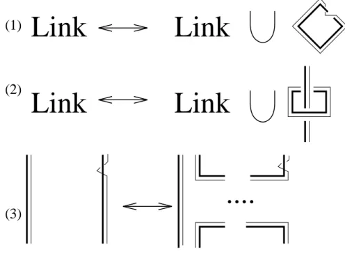
Definition 2.5

The following moves are called Kirby move (1) (2) (3).

(1) Insert or delete a component spanning an embedded disk with a longitude which meets the disk transversally once.

(2) Insert or delete a pair of components, one of which spans a disk meet- ing only the pair and its longitude does not meet this disk, the other of which intersects with the disk transversally once.

(3) Replace a component and its longitude by band sums of these and a longitude of another component.

....

(1)

(3)

(2) Link Link

Link Link

Figure 1: The Kirby move

In the above figure, the fat lines denote components of framed links and the thin lines denote longitudes of components.

The following theorem is proved in [1].

Theorem 2.6 Let L = l

∪ l

∪ · · · ∪ l

be a link in M and γ

be a longitude

of l

, (1 ≤ i ≤ n). Similarly, let L

= l

∪ l

∪ · · · ∪ l

be a link in M and

Definition 2.7

The group of orientation-preserving self homeomorphisms of Σ

modulo the subgroup of those which are isotopic to the identity map is called a mapping class group of Σ

.

Definition 2.8

Let c be a simple closed curve on Σ

. N (c) is parameterized by {(r, θ) | 1 ≤ r ≤ 2, θ ∈ R mod 2π}. A self homeomorphism of Σ

which is the identity on N(c) and is the map (r, θ) 7→ (r, θ − 2πr) on N (c) is called a Dehn twist along c.

It is denoted by τ

.

c c

Figure 2:

Let a

, b

, c

be following curves on Σ

.

....

1

1 1 2

2 2

g

g-1 g

a a

b c b c c b

a

Figure 3:

The following theorem is proved by W.B.R.Lickorish in [3].

Theorem 2.9 A mapping class group is generated by isotopy classes of (i) A

: a Dehn twist along a

, 1 ≤ i ≤ g

(ii) B

: a Dehn twist along b

, 1 ≤ j ≤ g

(iii) C

: a Dehn twist along c

, 1 ≤ k ≤ g − 1

Definition 2.10

Let N be a manifold with boundary, N

be a copy of N and B be a subset of

∂N . Then a manifold which is obtained from N ∪ B × [0, 1] ∪ N

by identifying

x ∈ B ⊂ N with (x, 0) ∈ B × [0, 1] and x

∈ B ⊂ N

with (x

, 1) ∈ B × [0, 1] is

called a double of N with respect to B. It is denoted by D

(N ). If B is equal

to ∂N , then we simply write D(N ). Note that D

(N) is homeomorphic to a

manifold which is obtained by removing {∂N \ B} × [0, 1] from D(N ).

3 Proof of Theorem 1.1

First, we prepare a technical lemma.

Let c be a simple closed curve on Σ

. We construct a 3-manifold by identifying (x,

) in Σ

× [0,

] with (τ

(x),

) in Σ

× [

, 1]. This 3-manifold is denoted by N

.

Lemma 3.1 Let c

be a simple closed curve c × {

−δ} in Σ

×[0,

] ⊂ N

, where δ is a positive constant. Let γ be a longitude of c

which is obtained by twisting one of simple closed curves appearing as ∂N (c

) ∩ Σ

× {

− δ} once in a left handed direction. Then N

(c

, γ) is homeomorphic to Σ

× [0, 1].

Proof

Let N (c) be a regular neighborhood of c such that τ

is the identity on Σ

\ intN(c). We choose positive constants ε, ε

such that N (c) × [

− ε,

− ε

] is a regular neighborhood of c

in N

. D denotes this subset of N

. Then, a map τ

× id : Σ

× [

− ε

,

] ⊂ N

→ Σ

× [

− ε

,

] ⊂ Σ

× [0, 1] is extended to a map h : N

\ intD → Σ

× [0, 1]. The complement of the image h(N

\ D) in Σ

× [0, 1]

is homeomorphic to a solid torus. The preimage of a meridian of this solid torus by h is isotopic to γ. Therefore N

(c

, γ) is homeomorphic to Σ

× [0, 1].

2

N(c)

h

Figure 4: h : N

\ intD → Σ

× [0, 1]

Remark 3.2

(1)By the proof of the above lemma, there is a natural identification between Σ

× {t} in N

and Σ

× {t} in Σ

× [0, 1].

(2)Let N

be a 3-manifold which is obtained by identifying (x,

) in Σ

× [0,

] with (τ

(x),

) in Σ

× [

, 1] and let c

be a simple closed curve c × {

− δ} in N

. Let γ

be a longitude which is obtained by twisting one of curves appearing as ∂N (c

) ∩ Σ

× {

− δ} once in a right handed direction. Then, it is proved in the same way that N

(c

, γ

) is homeomorphic to Σ

× [0, 1].

Proof of theorem 1.1

Suppose that a closed surface bundle M

is given. It follows from theorem 2.9 that an arbitrary self homeomorphism of Σ

is represented by a composition of a finite number of Dehn twists. Thus, we can choose simple closed curves c

, c

, · · · , c

on Σ

such that the monodromy ϕ is represented by τ

◦ τ

◦

· · · ◦ τ

, where ε

= ±1, (1 ≤ i ≤ m).

Step.1

In this step, we construct a link L

= l

∪ l

∪ · · · ∪ l

in M

and a longitude γ

of l

, (1 ≤ i ≤ m), such that M

(L

, {γ

}

) is homeomorphic to Σ

× S

.

M

= Σ

× [0, 1]/(x, 0) ∼ (ϕ(x), 1) is represented as follows. (x,

) in Σ

×

,

is identified with (τ

(x),

) in Σ

×

,

, (1 ≤ i ≤ m).

(x, 1) in Σ

×

, 1

is identified with (x, 0) in Σ

×

0,

.

Then a simple closed curve l

and a longitude γ

of l

are specified as in lemma 3.1, (1 ≤ i ≤ m). Let L

be a link l

∪ l

∪ · · · ∪ l

. Then M

(L

, {γ

}

) is homeomorphic to Σ

× S

. We remarked that each l

is on a fiber of M

. Step.2

In this step, we construct a link L

= l

∪l

∪· · ·∪l

in Σ

×S

and a longitude γ

of l

, (0 ≤ j ≤ 2g), such that {Σ

× S

}(L

, {γ

}

) is homeomorphic to S

.

Let l

be {x} × S

⊂ Σ

× S

. Let R

be a surface obtained by plumbing 2g copies of annuli. Then Σ

\ intN (x) is homeomorphic to R

. Σ

× S

\ intN (l

) is homeomorphic to R

× S

.

Note that Σ

× S

is homeomorphic to D(Σ

× [0, 1]). Let us decompose

∂(R

× [0, 1]) into two parts, B

= R

× {0, 1} and B

= {∂R

} × [0, 1]. Then

{Σ

× S

} \ intN (l

) is homeomorphic to D

(R

× [0, 1]). T

his R

× [0, 1] is homeomorphic to a handle body of genus 2g.

...

Figure 5: R

× [0, 1]

We divide R

× [0, 1] into following 2g solid tori H

, H

, · · · , H

.

H

B

H

H

B

H

H

B

H

B

...

D

Figure 6: H

, H

, · · · , H

We construct D

(H

). Let D be a disk on ∂H

which is identified with a disk on ∂H

. ∂H

consists of ∂H

∩ B

, ∂H

∩ B

and D. ∂D is decomposed into eight parts. Four parts appear as D ∩ ∂H

∩ B

. The other parts appear as D ∩ ∂H

∩ B

. These indicate that D

(D) is homeomorphic to a 4- punctured sphere. While ∂H

∩ B

has two connected components and each of them is homeomorphic to D

. The boundary of a component of ∂H

∩ B

is decomposed into four parts. Two parts appear as ∂H

∩ B

∩ B

. The other parts appear as ∂H

∩B

∩D. These indicate that D

(∂H

∩B

) has two connected components. Each of them is homeomorphic to an annulus, boundaries of which are attached to ∂D

(D).

Remark that a double of a solid torus is homeomorphic to S

× S

. Con-

sequently, D

(H

) is homeomorphic to a 3-manifold which is obtained by

removing the interior of a 3-ball with two 1-handles from S

× S

. The boundary of this 3-ball corresponds to D

(D) and the boundaries of these 1-handles correspond to D

(∂H

∩ B

).

identify

= S x [0,1] / (x,0) ~(x,1) S x S

2

Figure 7: D

(H

)

Similar construction shows that D

(H

) is homeomorphic to a 3-manifold illustrated in Figure 8, (1 ≤ j ≤ 2g). We put D

(H

) together, (1 ≤ j ≤ 2g ).

Since B

is homeomorphic to an annulus, D

(B

) is homeomorphic to a torus.

Therefore, D

(R

× [0, 1]) is homeomorphic to a 3-manifold which is obtained by removing the interior of a solid torus from a connected sum of 2g copies of S

× S

. The boundary of the solid torus corresponds to D

(B

).

....

paste paste

a solid torus is obtained by connecting these arcs

Figure 8: D

(R

× [0, 1])

Let γ

be a simple closed curve {y}×S

⊂ ∂N (x)×S

. This γ

is a longitude of l

such that {Σ

× S

}(l

, γ

) is homeomorphic to a connected sum of 2g copies of S

× S

.

{y} x [0,1]

R x [0,1]g

in the double γ’0

Figure 9: γ

Let l

∪ l

∪ · · · ∪ l

be a link and {γ

}

be longitudes illustrated in Figure 10. Then S

is obtained by a framed surgery on this link in a connected sum of 2g copies of S

× S

along {γ

}

.

γ’ γ’ γ’

....

paste paste

l’

l’ l’

1 2 2 3

3

Figure 10: l

∪ · · · ∪ l

We can regard this link as being in Σ

× S

. Let L

be a link l

∪ l

∪ · · · ∪ l

in Σ

× S

. Then, {Σ

× S

}(L

, {γ

}

) is homeomorphic to S

, where {γ

}

are longitudes specified as above.

We remark that each l

and γ

are regarded as being on R

×{t} ⊂ R

×[0, 1].

This means that l

and γ

are regarded as being on fibers of Σ

×S

, (1 ≤ j ≤ 2g ).

Step.3

In this step, we construct a link L in M

and longitudes {γ

}

such that each component of L intersects with a fiber of M

at only one point and M

(L, {γ

}

) is homeomorphic to S

.

We regard Σ

× S

as M

(L

, {γ

}

). We can chose L

in step.2 so that L

∩ L

= φ. Thus L

∪ L

is a link in M

. Note that M

(L

∪ L

, {γ

, . . . , γ

, γ

, γ

, . . . , γ

}) is homeomorphic to S

.

As we remarked before, each component of L

is on a fiber of M

. Since Σ

× {t} in M

is identified with that in Σ

× S

by remark 3.2, l

∪ · · · ∪ l

⊂ L

are regarded as being on fibers of M

. Then, we perform the Kirby move (3) to L

∪ L

. We replace each component of l

∪ · · · ∪ l

∪ l

∪ · · · ∪ l

by a band sum of the component and γ

. γ

intersects a fiber of M

at only one point and L

∪ L

\ l

is regarded as being on fibers of M

. Hence, we can slightly isotope the link obtained by this move such that each component intersects with a fiber of M

at only one point.

γ

’ l’

γ

’’

0 0

l’

a fiber of M

Figure 11: Kirby move (3)

Let L be this modified link in M

and {γ

}

be longitudes which obtained by the above moves from the longitudes specified in step.1 and 2, where n = m + 2g + 1.

Step.4

Let L

= l

∪ · · · ∪ l

be the dual link of (L, {γ

}

). S

\ L

is homeo- morphic to M

\ L. Thus, it admits a fibration over S

. To complete the proof, we have only to prove that L

is a fibred link in S

. This follows that the in- tersection of the fiber with a meridian of ∂N (l

) is only one point. However,

∂N (l

) is identified with ∂N (l

) and a meridian of ∂N (l

) is identified with γ

.

Hence the intersection of a fiber of M and γ

is only one point. Consequently,

4 Examples of framed link presentations

The aim of this section is to construct framed link presentations of surface bundles with given monodromies.

A framed link in the 3-sphere can be regarded as a link in the 3-sphere, each component of which is labeled by an integer in the following way. Let l be a component of the framed link in the 3-sphere. l is labeled 0 if a longitude of l is homologically 0 in S

\ l. l is labeled n if a longitude of l is obtained by twisting the longitude determined by 0 n times in a right handed direction. Note that the isotopy class of a longitude is determined by this integer.

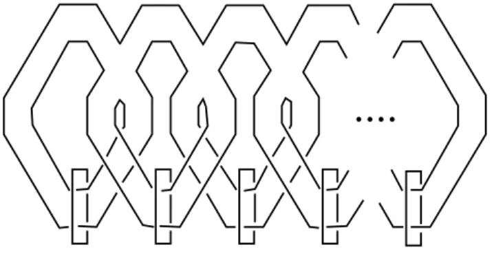
Example 4.1

The most simplest example is Σ

× S

. We remark that a framed link which represents this surface bundle is obtained in [4] by a different construction.

By tracing step.2 of the proof of theorem 1.1, we can illustrate the dual link of (L

, {γ

}

), where this is a framed link in Σ

× S

such that {Σ

× S

}(L

, {γ

}

) is homeomorphic to S

.

....

Figure 12: the dual link of (L

, {γ

}

)

This shows that the dual link with some framings represents Σ

× S

. The

framings are determined by the following way. l

⊂ L

intersects with a fiber of

Σ

× S

at only one point. Since the other component are regarded as being on

fibers of Σ

× S

, there is a fiber Σ

× {t} which Σ

× {t} ∩ L

= Σ

× {t} ∩ l

.

This implies that the longitude of l

which we want bounds a surface in S

\ L

.

Therefore, we label 0 to l

. The other component are also labeled by 0. Because

each of them with the framing which we want is a framed link presentation of

S

× S

.

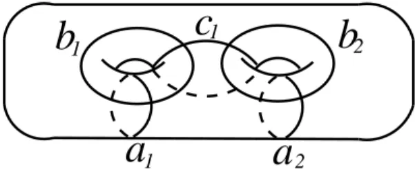
Example 4.2

Let A

, A

, B

, B

, C

be Dehn twists along following a

, a

, b

, b

, c

.

a a

c b

1

1 2

2

b

Figure 13:

We regard the curve b

illustrated above as being on a fiber of M

. Step.1 of the proof of theorem 1.1 shows that M

(b

, γ) is homeomorphic to Σ

× S

where γ is the longitude of b

specified in lemma 3.1. By the proof of lemma 3.1, we may suppose that the dual link b

is on a fiber of Σ

× S

. This b

can be regarded as in S

which is obtained by surgeries from Σ

× S

. We can determine the framing of b

by the proof of lemma 3.1. Hence we get a framed link presentation of M

.

0 0 0 0

0

1

Figure 14: A framed link which represents M

We can find framed links which represents M

, M

, M

, similarly. Framed links which represent M

, M

are the followings.

0 0 0 0

0

Figure 15: A framed link which represents M

0 0 0 0

1 1 0

Figure 16: A framed link which represents M

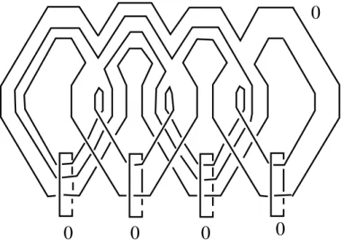
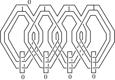
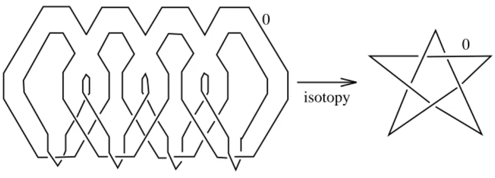
Example 4.3

Let ϕ be a self homeomorphism of Σ

such that

ϕ = A

C

B

B

(4.1)

Then a framed link which represents M

in our construction is illustrated in Figure 17.

0 0 0 0

0

1 1 1 1

Figure 17: a framed link which represents M

This is modified by Kirby moves to the (2,5) torus knot.

0 0 1

0

-1

0 0

0

1

isotopy Kirby

move (3) and (1)

Kirby

move

(3) x 2

and (1)

0 0

isotopy

Figure 19: a framed link which represents M

In the same way, if ϕ = A

B

· · · B

C

· · · C

then a framed link presentation of M

in our construction is modified by Kirby moves to a (2, 2g + 1) torus knot labeled 0.

Example 4.4

Let ϕ be a self homeomorphism of Σ

such that ϕ = A

A

2

C

B

B

(4.2)

We obtain a framed link which represents M

in our construction.

0 0 0 0

0 1

-1

Figure 20:

This is modified by Kirby moves to a framed knot.

0 1

0 1

0 0 0 0

1 1 1

-1

1

0 0

Figure 21:

Next proposition easily follows Example 4.4.

Proposition 4.5 Let A

, B

, C

be Dehn twists defined in Theorem 2.9 and ϕ be a self homeomorphism of Σ

. If ϕ is isotopic to A

◦ A

◦ B

◦ · · · ◦ B

◦ C

◦ · · · ◦ C

, where ε

, δ

= ±1, (1 ≤ i ≤ g), (1 ≤ j ≤ g − 1), λ

= −δ

and λ

is an arbitrary integer. Then the surface bundle with monodromy ϕ is

represented by a fibered knot in the 3-sphere labeled 0.

5 Surface bundles represented by fibered knots labeled 0

In this section, we discuss the problem of when a closed surface bundle M

is represented by a fibered knot with an induced framing. Note that the induced framing of a fibered knot is necessary 0.

The following is a well known theorem for the problem. Let ϕ be a self homeomorphism of Σ

. ϕ

denotes an automorphism of H

(Σ

) induced by ϕ.

ϕ

is regarded as an element of Sp

( Z ).

Theorem 5.1 If a closed surface bundle is represented by a fibered knot in the 3-sphere labeled 0, then the monodromy ϕ satisfies

det(ϕ

− I) = ±1 (5.1)

where I denotes the 2g × 2g unit matrix.

Proof

We shall prove that ϕ

− I is an automorphism of H

(Σ

). This induces det(ϕ

− I) = ±1.

If a closed surface bundle M

is represented by a fibered knot labeled 0, then there is a knot K in M

such that K intersects with a fiber at only one point and M

\K is embedded into S

. Since the first homology group of a knot complement in S

is Z, if M

\K is embedded into S

then H

(M

\ K) is Z. Moreover, since K intersects with a fiber at only one point, H

(M

\ K) is isomorphic to H

(M

). Consequently, if M

is represented by a fibered knot labeled 0, H

(M

) is Z.

C

(X ) denotes a chain complex of a topological space X. Let ˜ M

be an infinite cyclic cover of M

. Since M

is a fiber bundle over S

, there is a short exact sequence

0 −→ C

( ˜ M

) −→

C

( ˜ M

) −→ C

(M

) −→ 0 (5.2) where t is an automorphism of C

( ˜ M

) induced by a generator of the group of covering transformations. Note that ˜ M

is homotopy equivalent to Σ

. Then (5.2) induces a long exact sequence

· · · −→ H

(Σ

)

−→

H

(Σ

) −→

H

(M

) −→ H

(Σ

) −→ · · · (5.3) If H

(M

) is isomorphic to Z, then i

is a 0-map into H

(M

). It indicates that ϕ

− I is an automorphism of H

(Σ

).

2

Next, we observe that the condition (5.1) is sufficient for genus 1 case. This is a well known fact.

Proposition 5.2 A torus bundle with a monodromy ϕ is represented by a fibered knot in the 3-sphere labeled 0 if and only if ϕ satisfies det(ϕ

− I) = ±1.

In genus 1 case, an isotopy class of a self homeomorphism of T

is determined by its induced automorphism of H

(T

), see [6]. Hence, we identify a self home- omorphism of T

with an induced automorphism of H

(T

). Since H

(T

) is Z

, that is an element of SL

(Z).

Proof of Proposition 5.2

One direction comes from theorem 5.1.

The following claim shows that torus bundles of which monodromies satisfy the condition (5.1) are homeomorphic to either M

or M

, where L and R are following elements of SL

(Z).

L = 1 1 0 1

!

R = 1 0 1 1

!

Claim 1 Let X be an element of SL

(Z) such that detX = 1 and X-I is also an element of SL

(Z). Then X is conjugate to either LR or LR

.

Proof of Claim

Suppose that X is represented as the following.

a b c d

!

a, b, c, d ∈ Z If X in SL

(Z) satisfies det(X − I ) = ±1,

det a − 1 b c d − 1

!

= (a − 1)(d − 1) − bc

= ad − bc − (a + d) + 1 = ±1 a + d = 1 or 3

That is, trX = 1 or trX = 3.

Now, we prepare following four relations.

RXR

= 1 0 1 1

!

a b c d

!

1 0

−1 1

!

= a − b b

a − b + c − d b + d

!

R

XR = 1 0

−1 1

!

a b c d

!

1 0 1 1

!

= a + b b

−a − b + c + d −b + d

!

By using these relations, if min{|b|, |c|} is smaller than |a| then we can find X

conjugate to X such that (1,1)-entry of X

is non-negative and smaller than that of X. Hence we consider when min{|b|, |c|} is smaller than |a|.

Case 1. trX = 1

From a + d = 1 and ad − bc = 1,

bc = ad − 1 = −a

+ a − 1 (min{|b|, |c|})

≤ |bc| = | − a

+ a − 1|

If a ≥ 1, this induces min{|b|, |c|} ≤ a.

Case 2. trX = 3

From a + d = 3 and ad − bc = 1,

bc = ad − 1 = −a

+ 3a − 1 (min{|b|, |c|})

≤ |bc| = | − a

+ 3a − 1|

If a ≥ 3, this induces min{|b|, |c|} ≤ a.

Consequently, if X satisfies det(X−I) = ±1, X is conjugate to one of following matrices.

0 1

−1 1

!

= LR

0 −1

1 1

!

= L

R 0 1

−1 3

!

= R

LR

0 −1 1 3

!

= R

L

R 1 1 1 2

!

= RL 1 −1

−1 2

!

= R

L

2 1 1 1

!

= LR 2 −1

−1 1

!

= L

R

These are conjugate to either LR or LR

.

2 Then, it is well known that M

is represented by the figure-eight-knot labeled 0 in S

and M

is represented by the trefoil labeled 0 in S

, (See,[6]). It completes the proof of proposition 5.3.

2

References

[1] R.Fenn and C.Rourke, On kirby’s calculus of links, Topology. 18(1979). 1-15.

[2] W.B.R.Lickorish, A finite set of generators for the homeotopy group of a 2-manifold, Proc. Camb. Phil. Soc. 60(1964). 769-778.

[3] W.B.R.Lickorish, A presentation of orientable combinatorial 3-manifolds, Ann. of Math. (2) 76(1962). 531-540.

[4] J.M.Montesinos, Classical Tassellations and Three-Manifolds, Springer.

1987.

[5] A.W.Reid, A non-Haken hyperbolic 3-manifold covered by a surface bundle, To appear in Pacific J.Math.

[6] D.Rolfsen, Knots and Links, Publish or Perish, Berkeley,Ca.1976.

[7] W.P.Thurston, Three dimensional manifolds, Kleinian groups and hyper-

bolic geometry, Bull. A.M.S. 6(1982). 357-381.