Visualizing the Shape of Society: An Analysis of Public Bads and Burden Allocation due to 1
Household Consumption Using an Input-Output Approach 2
3
Andrew Chapman
1, Yosuke Shigetomi
24
5
1
International Institute for Carbon Neutral Energy Research (I2CNER). Kyushu University, 6
Fukuoka, Japan.
7
2
Graduate School of Fisheries and Environmental Sciences, Nagasaki University, Nagasaki 8
Japan.
9 10
Abstract 11
This study investigates how our lifestyles can cause societal issue including a reduction in 12
social equity due to the consumption of natural resources. Based on a range of household 13
environmental footprints and their application to a quantitative social equity evaluation 14
framework, a methodology is proposed which identifies the creation and origin of public bads 15
within society. This research builds on the methodologies of energy policy sustainability 16
evaluation incorporated with environmentally extended input output analysis in order to 17
critically assess lifestyle-based consumption impacts, and to quantify the allocation of 18
subsequent burdens across generations. Further, the proposed methodology is applied to a 19
case study in Japan, an aging, shrinking population. Analysis identifies the increasing burden 20
originating with elderly generations, and due to the resolution offered by the methodology, 21
specifically identifies commodities and services which underpin these future burdens, 22
allowing for policy implications to be drawn. The public bads and consumption burden 23
indicator established through the described methodology is proposed as a footprint 24
harmonizing tool to assess sustainability and supplement the footprint family.
25 26
Keywords: public bads, environmentally extended input-output analysis, footprint, household 27
consumption, social equity 28
29
1. Introduction 30
Our lifestyle choices require the consumption of resources to sustain, and this consumption 31
can be quantified in terms of the amount of capital expended, or alternatively in terms of the 32
amount and types of resources that people consume. When the resources that people consume 33
are limited in nature, imbalances can emerge between sectors of society, often dependent on 34
income or other socio-economic factors. Further, consumption of finite resources and energy 35
to sustain our lifestyles has flow-on impacts including the generation of social ills such as 36
pollution, and the depletion of critical materials. Ideally, the benefits and burdens within 37
society would be shared equitably, however, in the case of the environment, and the depletion 38
of finite materials, those who benefit most do not necessarily bear the burden that their 39
lifestyles entail (Johnson, 2012).
40
Japan, the focus of this study faces a combination of demographic issues including the highest 41
level of urbanization, the most rapidly aging population and among the lowest working age 42
population ratio when compared to its Asian peers and other nations with advanced 43
economies (Chomik & Piggott, 2015). In addition, as the fertility rate is also declining, the 44
population is shrinking, leading to a depletion in the labor force and negative impacts for the 45
economy at large (Muto et al, 2016). The national government of Japan are cognizant of the 46
demographic challenges at hand, and have identified the potential energy saving benefits that 47
a declining population engenders (METI, 2014). At the same time, the Strategic Energy Plan 48
(2014) recognizes that there are challenges ahead in coping with energy demand structure 49
changes and the incorporation of technological innovation, complemented by the Long-term 50
Energy Supply and Demand Outlook which takes into account demographic projections in 51
designing the primary energy supply structure to 2030 (METI, 2015).
52
The aim of this research is to identify the impact of household lifestyle on the creation of 53
public bads and environmental injustices between generations, and to assess this trend over 54
time, as the population of Japan not only shrinks, but also ages. This research takes a unique 55
analysis viewpoint, focusing on household lifestyle and consumption for household 56
generations between the ages of 20 and 70 (and above). This research assesses the resultant 57
generation of public bads such as air and land pollution from household waste, carbon dioxide 58
and particulate matter from energy consumption, and the level of limited material 59
consumption. Based on this assessment, the broader issues of environmental and energy 60
injustice and social ramifications are addressed. This research combines the analytical aspects 61
of household environmental footprints using environmentally extended input-output analysis 62
(EEIOA) and a modified application of social equity quantification and identification of 63
burden distribution.
64
65
2. Background and Literature Review 66
This research is underpinned by environmental and energy policy assessment methodologies 67
which consider lifestyle, consumption and social equity aspects. The three key concepts of 68
social equity, environmental justice and environmental footprints using EEIOA are detailed 69
below, including a review of precedential scholarship which informs the unique approach 70
proposed in this study.
71 72
2.1. Social Equity and Policy Burden 73
This research builds on existing research efforts to evaluate social equity as well as the burden 74
imparted on society through policy implementation. Such evaluative approaches are often 75
grouped within social impact-cognizant sustainability evaluations. Some examples include the 76
consideration of social equity within sustainable development (Campbell, 1996, Wheeler, 77
2002), the unequal impacts of climate change on lower income groups (Running, 2015), and 78
national sustainable energy transition policy studies for Germany (Joas et al., 2016), Japan 79
(Nesheiwat and Cross, 2013) and Italy (Magnani and Osti, 2016), among others, as well as 80
multi-nation comparative studies (Laes et al, 2014, Geels et al., 2016). More recently, the 81
emergence of the concept of energy justice has focused socially aware energy system research 82
on the three core tenets of distributive, procedural and recognition justice (McCauley et al., 83
2013, Heffron and McCauley, 2017). It is from this concept of energy justice, and a focus on 84
the distribution of costs and benefits due to the implementation of specific energy policies 85
(distributional justice) that the importance of social equity and its quantification was brought 86
to the fore (Chapman et al, 2016). Utilizing an investigation of specific energy policies in 87
various regions and at multiple scales including the solar feed-in tariff in Australia (Chapman 88
et al, 2016), participatory energy system scenario design at the national level, and social 89
outcomes of mega-solar siting at the regional level in Japan (Chapman and Pambudi, 2018, 90
Fraser and Chapman, 2018), the Energy Policy Sustainability Evaluation Framework (EPSEF) 91
was developed and refined using a number of social factors critical to energy policy. These 92
factors typically included energy cost increases, health, employment, participation, subsidy 93
allocation and greenhouse gas emissions, often using proxy indicators such as CO
2and PM
2.5, 94
among others.
95 96
2.2. Public Bads and Factors of Environmental Justice 97
This study addresses generational household consumption and its impact on social equity 98
outcomes, specifically identifying the creation of public bads which cause an inequitable or 99
unjust distribution of burdens across household generations. The investigation of public bad 100
generation and their final distribution across society has precedents in the environmental
101
justice movement, which seeks to identify and redress the disproportionate allocation of 102
environmental burdens or benefits which cause social inequality (Chakraborty, Collins, &
103
Grineski, 2016). Recent research has expanded the scope of environmental justice studies 104
beyond the unequal distribution of environmental ills, to incorporate the issues of 105
empowerment, social justice and public health (Capaccioli, Poderi, Bettega, & D’Andrea, 106
2017). This broadening of the research scope has led to a number of recent noteworthy studies 107
which underpin the design of this research in terms of factors investigated and scale, while 108
supporting its originality and contribution to the academic field. This study is concerned with 109
the emergence of public bads which impact upon lifestyles, generated as a result of household 110
consumption. In order to identify relevant factors for a comprehensive investigation of these 111
public bads, precedential literature is evaluated to elicit key factors and proxy indicators, 112
beginning with the health-related issue of air pollution. The literature identifies an example 113
of a national level investigation of China’s rapid growth and subsequent increase in air 114
pollution, which demonstrated flow-on impacts to self-reported health and happiness levels.
115
Although impacts varied according to income, education employment and other factors, lower 116
and middle-income groups were influenced by these factors more than the higher income 117
groups (Gu et al, 2017). A focused study on exposure to air pollutants (specifically particulate 118
matter) due to commuting and inequality between socio-economic groups was undertaken in 119
London, however this study found no systematic relationship between income and exposure, 120
with transportation type heavily influencing results (Rivas, Kumar, & Hagen-Zanker, 2017).
121
Considering water usage and the tenets of environmental Justice, Mahlanza et al’s South 122
African study clarifies the issues surrounding management of this limited resource (2016).
123
Specifically, they identify issues with regard to policy development and stakeholder 124
engagement and the expectation that access to water is a basic human right. Additionally, they 125
find that when water provision is insufficient, householder’s are forced to compromise on 126
livelihood decisions, particularly the most vulnerable groups within society (Mahlanza, 127
Ziervogel, & Scott, 2016). Waste, and particularly industrial waste, as addressed in this study, 128
has been considered at the national level in India, identifying urban percentage as a strong 129
predictor of waste generation, while also demonstrating that socially and economically 130
disadvantaged groups are significantly more likely to generate hazardous industrial waste. For 131
nations such as India undergoing rapid industrial development, the need to incorporate 132
economic justice ideals into waste management approaches was extolled (Basu & Chakraborty, 133
2016). The scarcity of rare metals is well understood, and their concentration in specific 134
geographic regions has led to the consideration of mining risk as a factor which can impact 135
negatively upon householder’s lifestyles. The fact that rare metals (this study focuses on 136
neodymium) have unique properties with regard to modern technological applications, and
137
suffer from a lack of alternatives, has led to research around global supply chains along with 138
the need to address technical, environmental, social and recycling challenges faced by these 139
materials (Golev et al., 2014).
140
Finally, with regard to the ethical consideration of intergenerational environmental justice 141
Almassi investigates the notion of a reparative justice approach to climate ethics which deems 142
climate exploitation and degradation as ‘wrong’, requiring redress for future generations 143
(2017). Although this study does not specifically consider redress activities, the trend of future 144
generational public bad creation is explored, leading to the potential for policy implication 145
identification or remediation strategies.
146
Building on this precedential research, this study investigates the combined impact on public 147
bad generation of five factors; an increase in greenhouse gas emissions (GHG), air pollution 148
(PM), industrial waste, water consumption and rare metal depletion. Each of these five factors 149
are impacted upon by household consumption, and the change in the level of impact is 150
investigated per household generation.
151 152
2.3. Environmental Footprints using Environmentally Extended Input-output Analysis 153
The data which underpins each of the five proposed factors is determined from the 154
perspective of environmental footprints, a suitable indicator to evaluate the life cycle 155
environmental load generated by final consumption. In other words, environmental footprints 156
measure how human consumption depends on either limited natural resources, or generates 157
waste, or both (Hoekstra and Wiedmann, 2014). Footprint indicators have been developed to 158
assess the various environmental issues (e.g. resource depletion), particularly climate change 159
focusing on carbon (GHG/CO
2) footprints during the past two decades (Fang et al., 2014).
160
The EEIOA has been widely adopted to quantify regional environmental footprints owing to 161
the methodological merit of ensuring system boundaries under the input-output table (IOT) 162
which is incomplete when implementing a conventional LCA approach (Suh and Huppes, 163
2005). There are precedential studies analyzing the footprint for environmental indicators 164
related to the five proposed factors; carbon footprint, air pollution footprint, water footprint, 165
waste footprint, and critical metal footprint, within EEIOA. Thus, a brief review of EEIOA 166
research is provided as it relates to the five indicators below.
167
Numerous studies have carried out EEIOA to quantify carbon footprints on various scales to 168
date (Munksgaard and Pedersen, 2000; Wiedmann, 2009; Hertwich and Peters, 2009;
169
Kanemoto et al., 2016; Wolfram et al., 2016; Hubacek et al., 2017; Malik et al., 2018;
170
Steininger et al., 2018). The carbon footprint concept is the most widespread when compared 171
with other footprint analysis within academia and society. Of interest, the globalization of 172
production and trade of manufactured goods and its impact on global GHG emissions was
173
discussed utilizing the carbon footprint as part of the fifth Annual Report from the 174
Intergovernmental Panel on Climate Change (IPCC AR5 WG3, 2014). This particular 175
application of the carbon footprint was based on Caldeira and Davis (2011) and Peters et al.
176
(2011).
177
Several studies have also analyzed the footprint of various air pollutants such as PM
10, PM
2.5, 178
carbonaceous aerosols (black carbon and organic carbon), sulfur oxides, nitrogen oxides and 179
volatile organic compounds (Nansai et al., 2003; Sugiyama et al., 2009; Guan et al., 2014; Lin 180
et al., 2014; Takahashi et al., 2014; Moran and Kanemoto, 2016; Nagashima et al., 2017;
181
Zhang et al., 2017). Takahashi et al. (2014) also estimated the health impact (number of 182
premature deaths) due to carbonaceous aerosols generated through the supply chain, based 183
on the final consumption of each country and region, taking account the source-receptor 184
relationship among them. Further, Zhang et al. (2017) elucidated the relationship between 185
the number of premature deaths caused by PM
2.5via international trade, showing the impacts 186
of transboundary PM
2.5pollution on global health.
187
With regard to the water footprint, linkages are identified with the virtual water concept 188
(Hoekstra and Chapagain, 2007). The water footprint considers rainwater for crop production 189
(green water), surface and ground water that evaporates or is incorporated into a product 190
(blue water), and water required to assimilate pollutants based on existing ambient water 191
quality standards (gray water) (Hoekstra and Mekonnen, 2012). Whilst the early approaches 192
to water footprints were of a bottom-up nature, EEIOA has been applied to quantifying the 193
water footprint of various regions as a top-down approach (Feng et al., 2011; Dong et al., 194
2013, 2014; Ono et al., 2015; Wang et al., 2016; Chen et al., 2017).
195
In order to assess the waste footprint, Nakamura and Kondo (2002) first introduced a new 196
hybrid LCA model termed the waste input-output (WIO) model, enabling an estimate of 197
waste generation associated with final consumption and waste treatment. Based on the IOA, 198
incorporating the concept of WIO, the structure of waste footprints was examined in Japan 199
(Kagawa et al., 2004; Kondo and Nakamura, 2005; Tsukui et al., 2015), Australia (Reynolds 200
et al. 2014; Fry et al., 2016), France (Beylot et al., 2016, 2017), and Taiwan (Liao et al., 2015).
201
Further, Tisserant et al. (2017) addressed the footprint of global solid waste.
202
The critical metal footprint quantifies the direct and indirect requirements of critical metals 203
in the same manner as the material footprint (Wiedmann et al., 2015). The securing of scarce 204
metals within rare earth elements is of great concern in terms of economic advantage and for 205
their applications within new energy technologies. For these reasons the assessment of metal 206
criticality has become prominent in recent years (Graedel et al., 2015). Based on the concept 207
of the material footprint and criticality assessment, Nansai et al. (2015) developed a 208
methodology for quantifying the mining risk of three critical metals (neodymium, cobalt, and
209
platinum) in mining countries underpinning global consumption. They adopted the EEIOA 210
with an economy-wide material flow analysis (IO-MFA) (Nakamura et al., 2007). In a similar 211
manner, Nansai et al. (2017) assessed the supply risk of these metals generated at post-mining 212
stage implying the direct and indirect vulnerability of the Japanese economy to such a risk.
213
Nakajima et al. (2017) quantified the global land-use change derived from nickel consumption 214
in Japan based on the IO-MFA with statistic data of land-use. These were expressed as 215
footprint indicators.
216 217
2.4. Multiple Footprint Derivation from Household Consumption 218
Household consumption is the main driver of various footprints which are derived from final 219
demands, particularly in developed nations (Hertwich et al., 2011; Ivanova et al., 2016).
220
EEIOA is often applied to quantifying environmental footprints, mostly the carbon footprint, 221
derived from household consumption as a proxy of lifestyle (Zhang et al., 2015). In-depth 222
studies of household environmental footprints have been carried out using EEIOA in 223
conjunction with a consumption expenditure survey focusing on the age of the household 224
head and income distribution since the 2000’s (e.g. Wier et al., 2001; Webber and Matthews, 225
2008; Jones and Kammen, 2011; Chitnis et al., 2014; Wiedenhofer et al., 2017). The older 226
people, for example, generally consume more household heat and energy than the younger 227
people because they tend to stay longer in their houses and feel more sensitive to the 228
temperature than younger people. Younger people are more likely to consume to support the 229
cost of their private vehicle and for the cost of information and communications than older 230
people. These differences in lifestyle mainly relate to direct energy consumption from 231
households, and will affect the environmental footprint (Kronenberg, 2009; Shigetomi et al., 232
2014; 2015). There are several studies which reveal the differences arising from regional 233
household footprints due to differing lifestyles, household compositions, and geography 234
(Jonnes and Kammen, 2014; Baiocchi et al., 2015; Ivanova et al., 2017; Gill and Moeller, 2018).
235
In Japan, several precedential studies analyzed the structure of household carbon footprints 236
from similar perspectives (Shigetomi et al., 2014, 2018). In terms of studies which assess other 237
household footprints in Japan, Takase et al. (2005) quantified landfill consumption under 238
scenarios related to lifestyle changes while considering the life cycle up to the disposal stage 239
for each scenario using the WIO model. Shigetomi et al. (2015) estimated the impact of future 240
demographic trends on three critical metal footprints from 2005 to 2035 in Japan. Further, 241
Shigetomi et al. (2016) examined the trade-off between carbon and critical metal footprints 242
of Japanese households.
243
While the environmental footprint is an indicator which can represent single environmental 244
loads, it has also been adapted to simultaneously assess several footprints within the same
245
system (Ewing et al., 2012; Steen-Olsen et al., 2012; Tukker et al., 2016; Ivanova et al., 2017;
246
Simas et al., 2017; Tian et al., 2017). In this sense, the application of a “footprint family” that 247
considers more than one footprint indicator has been promoted as a way to develop 248
sustainable and interdisciplinary policy measures within the European Commission (Galli et 249
al., 2012, 2013; Fang et al., 2014). An examination of the potential complementary linkages 250
between the footprint family concept and the planetary boundary (Steffen et al., 2015) to 251
explore the gaps in environmental sustainability at the global scale (Fang et al., 2015).
252
In the next section, the methodology used to estimate public bads generated from Japanese 253
households by incorporating the EEIOA approach (augmented by an embodied PM
2.5254
emissions study), with the EPSEF is elaborated. To the best of the author’s knowledge, no 255
research to date has visualized and discussed the negative social equity impacts of household 256
consumption integrating an environmental footprint evaluation approach.
257 258
3. Methodology 259
This research combines the environmental evaluation methodologies of EEIOA and the 260
EPSEF in order to holistically evaluate lifestyle and consumption impacts on social equity by 261
measuring the creation of public bads and the resultant burden imparted between 2005 and 262
2035 in Japan.
263
The EPSEF was originally employed to quantify and distribute social equity outcomes across 264
income levels, to determine both the efficacy and the fairness of varying policy approaches or 265
technological interventions. In order to make these assessments, the EPSEF relies on a range 266
of factors, perceived to be important to stakeholders, which underpin social equity, as well as 267
detailed data regarding societal demographics. For this study, the EPSEF is modified to 268
express the creation of public bads resulting from household consumption across generations.
269
In addition, the origin of these public bads is investigated to determine which household 270
generations are exerting burden on society over time, and which generations bear this burden.
271
The public bads investigated in this research build on and integrate the author’s previous 272
social equity quantification and household footprinting research in line with precedential 273
literature, aiming to link the concepts of public bad creation and resultant environmental 274
injustices arising between household generations.
275
Thanks to a significant historical progression of EEIOA studies in Japan, databases for 276
embodied environmental load intensities (direct and indirect loads per monetary unit) are 277
plentiful, enabling the assessment of various footprints of household consumption based on 278
the Japanese IOT (JIOT) of 2005 (MIC, 2009). Using these established resources can 279
comprehensively cover estimates of the footprints corresponding to the four factors of GHG, 280
water, waste and mining risk for the critical metal selected in this study. Only the embodied
281
intensity for PM
2.5emissions is not yet established. Therefore, it is necessary to create this 282
resource to enable the proposed study.
283
The methodology is in 3 parts: 1) Public bads factor definition, 2) Estimation of household 284
footprints including the derivation of consumption induced PM
2.5emissions, and, 3) 285
Application of (2) to the modified EPSEF to be expressed in terms of public bads and the 286
consumption burden imparted by the lifestyle of household generations in Japan.
287 288
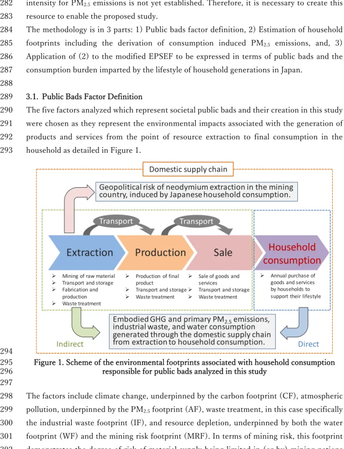
3.1. Public Bads Factor Definition 289
The five factors analyzed which represent societal public bads and their creation in this study 290
were chosen as they represent the environmental impacts associated with the generation of 291
products and services from the point of resource extraction to final consumption in the 292
household as detailed in Figure 1.
293
294
Figure 1. Scheme of the environmental footprints associated with household consumption 295
responsible for public bads analyzed in this study 296
297
The factors include climate change, underpinned by the carbon footprint (CF), atmospheric 298
pollution, underpinned by the PM
2.5footprint (AF), waste treatment, in this case specifically 299
the industrial waste footprint (IF), and resource depletion, underpinned by both the water 300
footprint (WF) and the mining risk footprint (MRF). In terms of mining risk, this footprint 301
demonstrates the degree of risk of material supply being limited in (or by) mining nations 302
(Nansai et al., 2015). Neodymium (Nd) is selected in this study due to its use in modern 303
technological devices, ranging from communications and ICT devices through to renewable 304
Geopolitical risk of neodymium extraction in the mining country, induced by Japanese household consumption.
Domestic supply chain
Production
Extraction Sale Household
consumption
Mining of raw material
Transport and storage
Fabrication and production
Waste treatment
Production of final product
Transport and storage
Waste treatment
Sale of goods and services
Transport and storage
Waste treatment
Transport Transport
Embodied GHG and primary PM
2.5emissions, industrial waste, and water consumption generated through the domestic supply chain from extraction to household consumption.
Indirect Direct
Annual purchase of goods and services by households to support their lifestyle
energy technology such as wind turbines, and a motor for electric vehicles (Shigetomi et al., 305
2017).
306
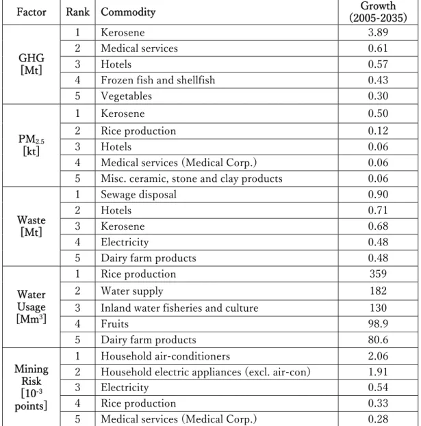
Table 1 outlines the public bads, specific factors, and footprints analyzed within this study.
307 308
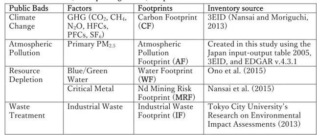
Table 1. Public bads, underpinning factors, footprints and data sources.
309
Public Bads Factors Footprints Inventory source Climate
Change
GHG (CO
2, CH
4, N
2O, HFCs, PFCs, SF
6)
Carbon Footprint (CF)
3EID (Nansai and Moriguchi, 2013)
Atmospheric Pollution
Primary PM
2.5Atmospheric Pollution Footprint (AF)
Created in this study using the Japan input-output table 2005, 3EID, and EDGAR v.4.3.1 Resource
Depletion
Blue/Green Water
Water Footprint (WF)
Ono et al. (2015) Critical Metal Nd Mining Risk
Footprint (MRF)
Nansai et al. (2015) Waste
Treatment
Industrial Waste Industrial Waste Footprint (IF)
Tokyo City University’s Research on Environmental Impact Assessments (2013) 310
3.2. Estimating Household Footprints to Determine Public Bads Factor Values 311
As detailed in the literature review and summarized in Table 1, all factors critical to this 312
research are derived through an application of EEIOA based on existing data sources, except 313
for PM
2.5. 314
The CF, AF, IF, WF, and MRF of household are quantified using the household consumption 315
expenditure of Japan based on the consumer expenditure survey, the 2005 JIOT, and the 316
embodied (direct and indirect) GHG emissions, PM
2.5emissions, industrial waste generation, 317
green and blue water consumption, and mining risk score for neodymium per unit of 318
expenditure; the so-called footprint intensity. The basic formula for calculating the household 319
environmental footprint based on EEIOA is as shown in Eq. (1).
320
( ˆ ˆ )
house= +
U d eL y (1)
321
where U and y
houseconsist of the targeted environmental footprint vector and household 322
final demand vector respectively. Vector d ˆ contains the elements of the amount of 323
environmental load directly generated from households per unit of expenditure. Vector e ˆ
324
represents the amount of direct environmental load per unit of expenditure from goods and 325
services (commodities). L denotes the Leontief inverse matrix (Millar and Blair, 2009), as 326
represented in Eq. (2).
327
( )
−1= −
L I A (2)
328
where I and A denote the identity matrix and the coefficient matrix derived from the IOT.
329
Thus, ( d eL ˆ ˆ + ) represents the footprint intensity. Focused on the public bads generated in 330
the consumer country, Eqs. (1) and (2) are rewritten using vector M ˆ containing the 331
elements of the ratio of imported commodities to quantify the domestic environmental 332
footprints U
domesticas follows:
333
( )( )
domestic
house
ˆ ˆ ′ ˆ
= + −
U d eL I M y (3)
334
( )
( ˆ )
−1′ = − −
L I I M A (4)
335
In this study, the CF intensity relies on the Embodied Energy and Emission Intensity Data for 336
Japan Using Input-Output Tables (3EID; Nansai and Moriguchi, 2013) and the Energy 337
Balance Table (METI, 2016). The direct household GHG (e.g. household heating, cooking, 338
and driving a passenger car) was estimated using the emission factors for energy commodities 339
(gasoline, kerosene, liquefied natural gas (LPG), city gas, electricity, and the other petroleum 340
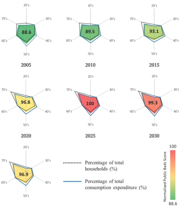
products) and its consumption share in line with the Energy Balance Table. The IF and WF 341
intensities reference Tokyo City University’s Research on Environmental Impact Assessments 342
(2013) and Ono et al. (2015), respectively. The MRF intensity used in this study, is derived 343
from the GLIO model (Nansai et al., 2009) that specifies the global supply chains of Japanese 344
commodities based on the JIOT (Nansai et al., 2015). Direct household water usage is 345
considered in the WF inventory. Because the industrial pollutions and neodymium mining are 346
not created directly by households, those direct loads are not estimated per unit of expenditure.
347
Further, because neodymium is not mined in Japan, the supply risk associated with domestic 348
commodities consumed by households throughout the global supply chain is observed.
349
With respect to the AF intensity, the sectoral PM
2.5emissions in Japan are incorporated using 350
the Emission Database for Global Atmospheric Research (EDGAR) v.4.3.1 (European 351
Commission, 2016) in coordination with the JIOT. EDGAR provides the annual amount of 352
primary PM
2.5emitted directly from 25 sectors for the period 1970-2010 according to the 353
IPCC 1996 standard. First, the amount of direct PM
2.5emissions from households was 354
estimated by multiplying the emission amounts from “1A4: Residential and other sectors” by 355
the percentage of direct energy consumption by the residential sector per summation of direct 356
energy consumption by both residential and commercial sectors, referring to the Energy 357
Balance Table (METI, 2016). Because direct emissions are generated from households 358
through the usage of kerosene for heating, the direct emissions intensity for household 359
consumption is also calculated by dividing the amount of the direct emissions by the total 360
output of kerosene on the JIOT. In addition, residual PM
2.5emissions (the emission by “1A4:
361
Residential and other sectors” minus the emission of the residential sector calculated above)
362
are defined as those which were emitted from commercial activities, used to estimate the 363
indirect PM
2.5emissions as follows.
364
In order to estimate indirect emissions, the 25 sectors within EDGAR were mapped to 365
approximately 400 commodities contained within the JIOT. Next, the sectoral PM
2.5366
emissions reported within EDGAR were allocated onto the corresponding commodities with 367
respect to direct energy consumption by commodity, referred to within 3EID. In the same 368
manner as for the direct emission intensity from households, the direct emission intensity 369
arising from commodities were calculated by dividing the amount of direct emissions by the 370
total output of the corresponding commodity within the JIOT. Finally, the direct emission 371
intensities of commodities were multiplied with the Leontief inverse matrix of the JIOT, 372
resulting in the indirect PM
2.5emissions intensity.
373
In order to obtain consumption expenditure by household attribute (in this case using the age 374
of the household head: 20’s; ≤29, 30’s; 30-39, 40’s; 40-49, 50’s; 50-59, 60’s; 60-69, 70’s; ≥70) 375
for calculation of footprints during the target period, the method used in previous studies 376
(Shigetomi et al. 2014; 2015; 2016) can be applied. Overall, the breakdown of consumption 377
expenditure consists of approximately 400 commodity sectors consistent with the JIOT. The 378
estimation of consumption expenditure is made with respect to demographic trends 379
anticipated by the national population census of Japan (National Institute of Population Social 380
Security Research, Population Statistics of Japan, 2013) and the consumer expenditure survey 381
(MIC, 2009). Finally, factors other than demographic trends such as technology were assumed 382
not to change from 2005 onwards under the estimation. The limitations of such an approach 383
are detailed in Section 5.3.
384 385
3.3. EPSEF Public Bads and Consumption Burden Application 386
Following the derivation of consumption-based environmental loads for each household 387
generation within the time period ranging from 2005-2035, the EPSEF is employed to 388
calculate the relative public bads creation across household generations, which, in 389
combination consumption per generation, can identify an overall ‘public bads score’ as well 390
as the origin of these bads, expressed as the ‘consumption burden’ for each timeframe 391
analyzed. The calculations are based on the EEIOA footprint results, according to the 392
following formulae:
393
Firstly, the household footprints are normalized thus:
394
𝐸𝑉
( )=
( )
( )
(5)
395
where EV is the normalized household footprint value, HF are the household footprints, with
396
i , and t representing the types of household footprint, and the analyzed timeframe 397
respectively.
398 399
Second, the normalized household footprint values for each time period are summed and the 400
relative public bads score can be calculated, including a factor for weighting of consumers 401
perceived importance of each footprint, thus:
402
𝑟𝑃𝐵
( )=
∑ ×( )
∑
(6)
403 404
where rPB is the relative public bads score, and w is the weighting score for each of the 405
footprints. Weighting of footprints is usually achieved through a survey of relevant 406
stakeholders, as undertaken in previous studies (e.g. Chapman et al, 2018). For the purposes 407
of this study, which is to demonstrate the development of a novel indicator, each of the 408
footprints are weighed equally ( w =1), however ideally, future jurisdiction specific studies 409
would include the stakeholder determined importance weightings for each investigated 410
footprint.
411
Third, the household expenditure ratio is derived as follows:
412
𝐸𝑅
( )=
( )
∑ ( )
(7)
413
where ER is the household expenditure ratio, and F is the total final consumption expenditure 414
by household generation.
415
Finally, for each of the household generations ( j ), the household expenditure ratio and relative 416
public bads values are plotted to form a polygon, from which the area weighted centroid is 417
derived (using geometric decomposition) to inform the consumption burden (x value) and 418
public bads score (y value).
419 420
4. Results and Discussion 421
In the following section the estimated footprints are detailed for each of the five public bads 422
underpinning factors from 2005-2035. This is followed by a visualization and discussion of 423
the results yielded by the EPSEF in its application to the public bads score calculation for each 424
time period, along with a consumption burden calculation. Advantages and limitations of the 425
proposed methodology are also addressed.
426 427
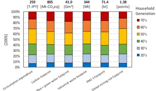
4.1. Household Environmental Footprints 428
The footprints for each of the public bad factors explored in this study are shown in Figure 2
429
using actual data from 2005. Households in their 50’s caused the greatest contribution toward 430
consumption expenditure among all of the footprints, followed by those in their 40’s and 60’s.
431
This is due to not only consumption trends, but also heavily influenced by the relatively large 432
number of households in their 40’s, 50’s and 60’s compared to other age groups in Japan. As 433
Japan ages, and the number of children being born decreases, it is likely that this trend will be 434
exacerbated.
435 436
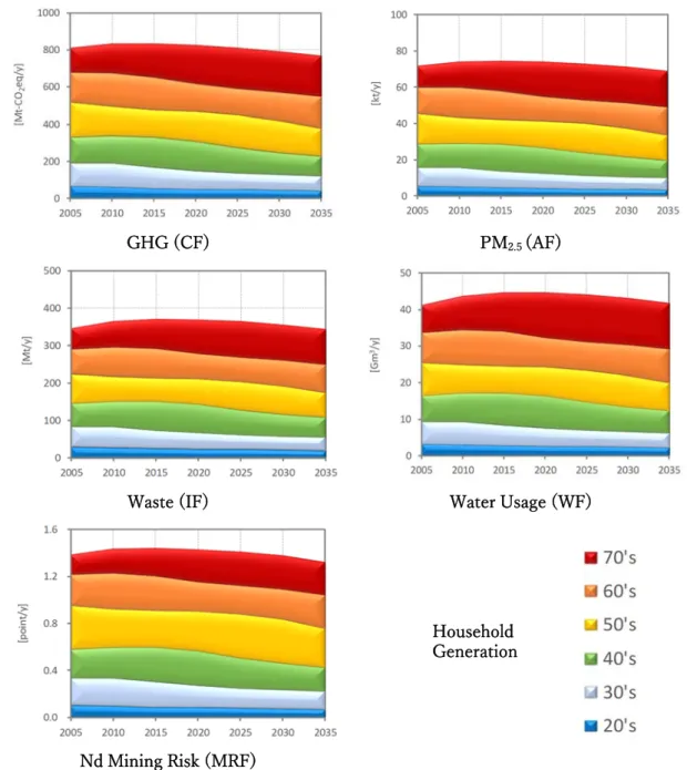
Total consumption expenditure first increases until 2010, and then drops over time, 437
approximately 9.9% by 2035 when compared to 2005 levels, under the assumptions outlined 438
in the methodology. Using these assumptions, Figure 3 details the trends of each footprint 439
and household generation, projected to 2035.
440 441
Figure 2. Scheme of the environmental footprints associated with household consumption responsible for public bads analyzed in this study in 2005
0%
10%
20%
30%
40%
50%
60%
70%
80%
90%
100%
70's 60's 50's 40's 30's 20's 805
[Mt-CO2eq]
41.0 [Gm3] 259
[T-JPY]
344 [Mt]
71.4 [kt]
1.38
[points] Household Generation
[2005]
442
GHG (CF) PM
2.5(AF)
Waste (IF) Water Usage (WF)
Household
.Generation
Nd Mining Risk (MRF)
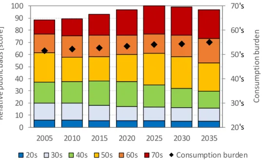
Figure 3. Footprints by household generation 2005-2035 443
Each of the footprints peak around the year 2015. In 2035, the CF is expected to be 5.1%
444
lower than in 2005, showing the largest decrease compared with other footprints. The MRF 445
and AF are projected to decrease by 4.4% and 4.0% respectively, while the decrease in IF is 446
negligible between 2005-2035. In 2035 only the WF is expected to be higher than in 2005.
447
With regard to the generational contributions, households in their 60’s and 70’s become most 448
influential toward the year 2035 for all footprints. For instance, elderly household’s 449
contributions account for 42-52% of the total footprints, while those in their 20’s and 30’s 450
only account for 14-15%. This result reflects the Japanese demographic shift into the future,
451
where an aging, shrinking society will increase the average age of households, due to a larger 452
number of households in their 60’s and 70’s. Reducing population, particularly due to low 453
child birth rates mean that in 2035, the relative number of households in their 20’s and 30’s 454
will be even lower than today, exacerbating this gap in terms of consumption and contribution 455
to footprints. In particular, during the period investigated, contributions from households in 456
their 70’s will grow markedly, becoming the largest CF, AF, IF and WF by household 457
generation in 2025. With regard to the MRF, households in their 50’s account for the largest 458
footprint per household generation in the year 2005.
459 460
4.2. Public Bads and Consumption Burden 461
First, the public bads score for each of the time periods investigated is shown in Figure 4. The 462
dotted line represents the number of households in each age group, while the blue line 463
expresses the percentage of consumption occurring in each group. Public bads are 464
represented by the colored polygon, expressing the overall amount of public bads by the color 465
shade, while the percentage of public bads originating from each age group is represented by 466
the polygon shape.
467
468
469
2005 2010 2015
2020 2025 2030
2035
Figure 4. Public Bads Score, Household and Consumption Distribution.
470 471
Imbalance in the ‘shape’ of society can be observed where consumption exceeds the 472
percentage of households in certain household generations, and likewise for the generation of 473
public bads. The public bads score begins at its lowest level in 2005, increasing steadily to a 474
peak in 2025, before returning to moderate levels similar to 2020, by 2035. The Japanese 475
population, predominantly in the 70’s and above age group grows steadily to 2035.
476
20's
30's
40's
50's 60's
70's
88.6
20's
30's
40's
50's 60's
70's
89.5
20's
30's
40's
50's 60's
70's
93.1
20's
30's
40's
50's 60's
70's
96.8
20's
30's
40's
50's 60's
70's
100
20's
30's
40's
50's 60's
70's
99.3
20's
30's
40's
50's 60's
70's
96.9
100
NormalizedPublic BadsScore 88.6