Experimental Study on Indices to Detect Damage of RC Beam Based on Fourier Analysis of Response to Impact Excitation

Experimental Study on Indices to Detect Damage of RC Beam Based on Fourier Analysis of Response to Impact Excitation

__________________________________________________________________________________________________________

AKIYO SANO, YUIKO KUMAGAI, AND MASAYUKI KOHIYAMA

ABSTRACT:

Regarding damage detection of reinforced concrete (RC) structure using an impact hammer and a piezoelectric acceleration sensor, experiment and analysis were carried out to propose a reliable index to assess severity of damage to a member of RC structure. A test piece of a RC beam was used. First, the test piece was simply supported and two vertical downward forces were loaded monotonically to damage it. At some stage of damage severity, the test piece was moved out from the loading apparatus, and then was supported by urethane bearings. After that with an impact hammer, an impulse wave was given on the surface of the test piece in which downward forces were applied. The vibration (acceleration) of the normal direction of the surface was measured by the six accelerometers that were placed on the loaded and impact excited surface. Impact excitation was conducted at seven points. The above set of processes of loading (damaging) and measuring response to impact excitation was repeated until the test piece exhibited multiple visible cracks from the bottom to the top of the beam. The accelerograms were analyzed by the Fourier transform and some indices using not only the Fourier amplitude spectrum but also the Fourier phase spectrum were examined on the applicability for detecting damage.

INTRODUCTION

If building structures or infrastructures become aged or deteriorated, concern for earthquake resistance increases. Health monitoring or diagnosis of a structure is conducted to evaluate the structural performance and to assess necessity of repair work.

When a structure is diagnosed by visual inspection, it is often difficult to find minor cracks or damage in interior parts. Hence it is desired to devise a technique to detect such minor damage and deterioration.

Neild et al. (2003)[1] propose a method to detect damage of a reinforced concrete (RC) beam, which is based on the nonlinear vibration characteristic between _____________

Graduate School of Science and Technology, Keio University

email address: [email protected]

vibration amplitude and the fundamental frequency. They conducted a cyclic loading test of a RC beam and measured the vibration response to impact excitation with an impact hammer. A clear change in the nonlinear vibration behavior was observed after experiencing very minor damage caused by a load less than 10% of the failure load.

However, they mention that the load is very small, and consequently, the method is unlikely suitable for detecting damage in RC bridges.

Ikeshita and Kitagawa (2005)[2] carried out an experiment on identification of damage location of a concrete test piece using an impact hammer. They focus on wave characteristic, especially on a Fourier amplitude spectrum of measured wave. In the experiment, although the method is aimed for damage detection of a RC structure, the test piece had no reinforcement, and damage was imitated by a relatively large notch, which was different from typical damage of a RC structure.

In this study, to propose a reliable index to assess severity of damage to a member of RC structure, the following experiment is conducted: a test piece of a RC beam is gradually damaged by static loading and bending cracks are generated. Then, responses to impact excitation with an impact hammer are measured. The accelerograms are analyzed by the Fourier transform and some indices using not only the Fourier amplitude spectrum but also the Fourier phase spectrum are examined on the applicability for detecting damage.

DAMAGE DETECTION EXPERIMENT

Experiment method

A test piece of a RC beam that has the dimension of 140×140×1100 mm was used as shown in Fig. 1. The concrete strength f

c

= 23.8 N/mm

²

(at 42 days) and the experiment was done at 61 days after concrete placing; the concrete characteristic is listed in Table 1.

Fig. 2 depicts the bar arrangement: D13-SD295A deformed bars (nominal diameter 13 mm) and φ 6-SD295A (diameter 6 mm) were used for the main and shear reinforcing bars, respectively.

Figure 1: A test piece of a RC beam.

1100

300 300 300

100 100

60 60

140

100

1100

300 300 300

100 100

60 60

140

100

Figure 2: Arrangement of bars.

Table 1: Characteristics of the concrete.

Modulus of longitudinal elasticity 2.24×10⁴ N/mm² Density 2.40×10³ kg/m³

Poisson's ratio 0.167

Compressive strength (at 42 days) 23.8 N/mm² Maximum dimension of coarse aggregate 20 mm

unit：mm 1100

300 300 300

100 Loading points 100

cross-section view 140

140

roller

unit：mm 1100

300 300 300

100 Loading points 100

cross-section view 140

140

cross-section view 140

140

roller

Figure 3: Loading condition.

First, the test piece was simply supported with the 900 mm span and two vertical downward forces were loaded monotonically to damage the test piece. The two forces were applied on the 300 mm-spaced points on the top of the test piece using a loading apparatus with a hydraulic cylinder (Fig. 3). The downward forces were measured by a load cell and the cracks of the test piece were observed by a microscope.

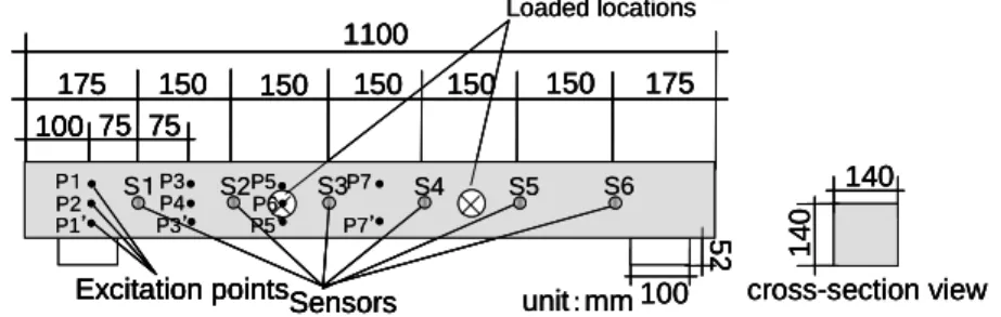
At some stage of damage severity, the test piece was moved out from the loading apparatus, and then was supported by urethane bearings after the test piece was turned 90 degrees around the longitudinal axis of the beam. After that, with an impact hammer, an impulse wave was given on the surface of the test piece that was originally the top, in which downward forces were applied. The vibration (acceleration) of the normal direction of the surface was measured by the six accelerometers that were placed on the loaded and impact excited surface as shown in Fig. 4. The sensors used were piezoelectric accelerometer of Model 2431 (Showa Sokki Corporation, frequency range:

0.5 to 20 kHz) and the sampling frequency was 10 kHz. Impact excitation was conducted at seven points (Fig. 4), and at each point, the excitation and measurement were repeated ten times.

The above process of loading (damaging) and measuring response to impact excitation was repeated until the test piece exhibited multiple visible cracks from the bottom to the top of the beam. The measurement was carried out for six stages in total.

The stages (damage levels) are named as follows: the condition without damage: C0, and conditions as damage progressed: C1, C2, C3, C4 and C5. Note that in the condition C3 the surface concrete of the excitation points was exfoliated due to the impacts, locations of the excitation points P1, P3, P5 and P7 were changed to P1’, P3’, P5’ and P7’, which were symmetric to the central longitudinal axis of the top of the test piece (Fig.4).

Figure 4: Locations of acceleration sensors and points of impact excitation.

Damage Condition

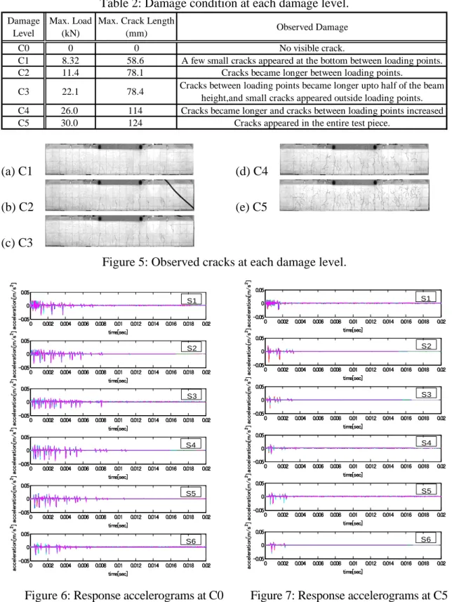
In the conditions C1 to C5, the cracks were observed as shown in Fig. 5. The cracks progressed and increased considerably from C3 to C4. Table 2 lists the total downward force, the maximum crack length, and the observed damage at each damage level. Fig. 6 and Fig. 7, show examples of the measured vibration by impact excitation in C0 and C5, respectively. An acceleration response to impact excitation at P1 (P1’ in C5) measured by the sensors S1 to S6 are compared in those figures.

Comparing Fig. 6 and Fig. 7, the strong amplitude of the acceleration continued for a long time (about 0.012 s) in C0 (no damage) while the acceleration attenuated soon in C5 (severely damaged). As damage progressed from C0 to C5, the duration of strong acceleration became shorter monotonically. This is arguably because wave propagation

cross-section view

140

1100

175 150 150 150 150 150 100

175 75 75

Sensors

Excitation points 100

52

140

unit：mm

P１

P6 P3 P4

P5 P2

P7

P1’ P3’ P5’ P7’

S１ S2 S3 S4 S5 S6

Loaded locations

cross-section view

140

cross-section view

140

1100

175 150 150 150 150 150 100

175 75 75

Sensors

Excitation points 100

52

140

unit：mm

P１

P6 P3 P4

P5 P2

P7

P1’ P3’ P5’ P7’

S１ S2 S3 S4 S5 S6

Loaded locations 1100

175 150 150 150 150 150 100

175 75 75

1100

175 150 150 150 150 150 100

175 75 75

Sensors Excitation pointsSensors

Excitation points 100

52

140

unit：mm

P１

P6 P3 P4

P5 P2

P7

P1’ P3’ P5’ P7’

S１ S2 S3 S4 S5 S6

P１

P6 P3 P4

P5 P2

P7

P1’ P3’ P5’ P7’

S１ S2 S3 S4 S5 S6

Loaded locations

was impeded by damage cracks, that is path of waves was cut off by the large cracks and the acceleration attenuated by friction and scattering due to the small cracks.

Table 2: Damage condition at each damage level.

Damage Level

Max. Load (kN)

Max. Crack Length

(mm) Observed Damage

C0 0 0 No visible crack.

C1 8.32 58.6 A few small cracks appeared at the bottom between loading points.

C2 11.4 78.1 Cracks became longer between loading points.

C3 22.1 78.4 Cracks between loading points became longer upto half of the beam height,and small cracks appeared outside loading points.

C4 26.0 114 Cracks became longer and cracks between loading points increased

C5 30.0 124 Cracks appeared in the entire test piece.

(a) C1 (b) C2 (c) C3

(d) C4 (e) C5

Figure 5: Observed cracks at each damage level.

0 0.002 0.004 0.006 0.008 0.01 0.012 0.014 0.016 0.018 0.02 -0.05

0 0.05

time[sec]

acceleration[m/s2]

0 0.002 0.004 0.006 0.008 0.01 0.012 0.014 0.016 0.018 0.02 -0.05

0 0.05

time[sec]

acceleration[m/s2]

0 0.002 0.004 0.006 0.008 0.01 0.012 0.014 0.016 0.018 0.02 -0.05

0 0.05

time[sec]

acceleration[m/s2]

0 0.002 0.004 0.006 0.008 0.01 0.012 0.014 0.016 0.018 0.02 -0.05

0 0.05

time[sec]

acceleration[m/s2]

0 0.002 0.004 0.006 0.008 0.01 0.012 0.014 0.016 0.018 0.02 -0.05

0 0.05

time[sec]

acceleration[m/s2]

0 0.002 0.004 0.006 0.008 0.01 0.012 0.014 0.016 0.018 0.02 -0.05

0 0.05

time[sec]

acceleration[m/s2]

S1

S2

S3

S4

S5

S6 0 0.002 0.004 0.006 0.008 0.01 0.012 0.014 0.016 0.018 0.02 -0.05

0 0.05

time[sec]

acceleration[m/s2]

0 0.002 0.004 0.006 0.008 0.01 0.012 0.014 0.016 0.018 0.02 -0.05

0 0.05

time[sec]

acceleration[m/s2]

0 0.002 0.004 0.006 0.008 0.01 0.012 0.014 0.016 0.018 0.02 -0.05

0 0.05

time[sec]

acceleration[m/s2]

0 0.002 0.004 0.006 0.008 0.01 0.012 0.014 0.016 0.018 0.02 -0.05

0 0.05

time[sec]

acceleration[m/s2]

0 0.002 0.004 0.006 0.008 0.01 0.012 0.014 0.016 0.018 0.02 -0.05

0 0.05

time[sec]

acceleration[m/s2]

0 0.002 0.004 0.006 0.008 0.01 0.012 0.014 0.016 0.018 0.02 -0.05

0 0.05

time[sec]

acceleration[m/s2]

S1

S2

S3

S4

S5

S6

0 0.002 0.004 0.006 0.008 0.01 0.012 0.014 0.016 0.018 0.02 -0.05

0 0.05

time[sec]

acceleration[m/s2]

0 0.002 0.004 0.006 0.008 0.01 0.012 0.014 0.016 0.018 0.02 -0.05

0 0.05

time[sec]

acceleration[m/s2]

0 0.002 0.004 0.006 0.008 0.01 0.012 0.014 0.016 0.018 0.02 -0.05

0 0.05

time[sec]

acceleration[m/s2]

0 0.002 0.004 0.006 0.008 0.01 0.012 0.014 0.016 0.018 0.02 -0.05

0 0.05

time[sec]

acceleration[m/s2]

0 0.002 0.004 0.006 0.008 0.01 0.012 0.014 0.016 0.018 0.02 -0.05

0 0.05

time[sec]

acceleration[m/s2]

0 0.002 0.004 0.006 0.008 0.01 0.012 0.014 0.016 0.018 0.02 -0.05

0 0.05

time[sec]

acceleration[m/s2]

S1

S2

S3

S4

S5

S6 0 0.002 0.004 0.006 0.008 0.01 0.012 0.014 0.016 0.018 0.02 -0.05

0 0.05

time[sec]

acceleration[m/s2]

0 0.002 0.004 0.006 0.008 0.01 0.012 0.014 0.016 0.018 0.02 -0.05

0 0.05

time[sec]

acceleration[m/s2]

0 0.002 0.004 0.006 0.008 0.01 0.012 0.014 0.016 0.018 0.02 -0.05

0 0.05

time[sec]

acceleration[m/s2]

0 0.002 0.004 0.006 0.008 0.01 0.012 0.014 0.016 0.018 0.02 -0.05

0 0.05

time[sec]

acceleration[m/s2]

0 0.002 0.004 0.006 0.008 0.01 0.012 0.014 0.016 0.018 0.02 -0.05

0 0.05

time[sec]

acceleration[m/s2]

0 0.002 0.004 0.006 0.008 0.01 0.012 0.014 0.016 0.018 0.02 -0.05

0 0.05

time[sec]

acceleration[m/s2]

S1

S2

S3

S4

S5

S6

Figure 6: Response accelerograms at C0 Figure 7: Response accelerograms at C5 (Excitation point: P1). (Excitation point: P1’).

ANALYSIS ON RELIABLE DAMAGE INDEX

Examined damage indices

To propose a reliable index to detect damage, several indices using Fourier spectrum of the measured acceleration were examined on the relation between damage level and value of those indices. In the analysis, five measured waves were selected from the ten at each excitation point in each damage level based on the signal to noise ratio of the accelerogram, the sufficient force level of the impact excitation, and hammering condition (double hammering data were eliminated). At damage level C2, double hammering occurred frequently, only three waves were available at excitation point P5, and only one at P7, which was possibly due to an exfoliation of concrete.

In this study, the following three indices were compared to detect damage: μ

1

and μ

2

, which are indices based on the Fourier amplitude spectrum of the accelerogram, and μ

3

based on the Fourier phase spectrum. The index μ

1

is defined by

( ^{( ) |} ) ^{/ max} ( ^{( )} )

1

= max A f f

_L

≤ f ≤ f

_H

P

_h

t

μ where f

_L

= 0.1×10

⁴

Hz, f

_H

= 1.2×10

⁴

Hz, and P

h

(t) is the time history of the force of impact excitation, in which compression force is positive (Fig.8). The Lower limit of the frequency range f

_L

was determined to ignore a direct current component at 0 Hz. The upper limit f

H

was determined by considering the time for the impact excitation wave to return to the top of the test piece after reflecting at the bottom. The shortest path of the reflected wave, dmin, is about the twice of the height of the test piece (140 mm), that is

d_min ≈0.28

m. The velocity of longitudinal wave Vp is:

m/s ) 3300

2 )(1 (1

) 1

( − × ≈

= ρ

V

_p

E

ν

－

＋ν ν

where the Young’s modulus of the concrete E ≈ 20 GPa, the density 10

3

4 . 2 ×

ρ ≈ kg/m

³

, the Poisson’s ratio

ν≈1/6

. Hence the time for the wave to return for the first time, t

ref

, and the frequency of arrival of the reflected wave, f

ref

, are:

= ^min ≈8.5×10^−5ｓ=85μ^ｓ

p

ref V

t d

and

1 1.2 10₄ Hz

×

≈

=

ref

ref t

f

, respectively.

Based on the above, the upper limit f

H

was assigned by f

ref

.

The index μ

2

is defined by μ

₂

= A ( f ) / max ( P

_h

( t ) ) where A ( f ) is the average of the Fourier amplitude spectrum between frequency range from

f_L

to

f_H

. The index μ

3

is the slope of the regression line for the unwrapped Fourier phase spectrum. The index μ

3

is considered to be proportional to group delay. The unwrapping process is to add

±2n

π (n is an integer) to phase φ

_i

so that the values of the phase φ

_i

might become continuous.

0 0.2 0.4 0.6 0.8 1

x 10^-3 0

0.005 0.01 0.015

time [s]

compression force [N]

Figure 8: Time history of the impact excitation.

Maximum compression force

Analysis of indices based on Fourier amplitude spectrum

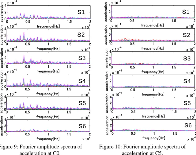
The Fourier amplitude spectra of the accelerograms observed at the damage levels C0 and C5 are shown in Fig.9 and Fig.10, respectively. The amplitude of low frequency range became smaller, The severer the damage level was. The same trend was observed at all the excitation point.

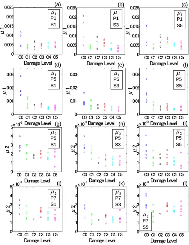
The distributions of the indices μ

1

and μ

2

are shown in Fig.11. Note that there was no consistent tendency at excitation point P3 in all sensors, possibly due to influence of the arrangement of rebars, and the results regarding P3 was disregarded.

Further study is required and planned to explain this result based on the FEM.

With respect to the index μ

₁

, comparing damage level C0 to C1, the value decreased at all the excitation points and the sensors. Consequently, a reliable threshold value can be set between damage level C0 and C1. Regarding the index μ

2

, similarly there was clear value change between damage levels C0 and C1 with respect to the excitation points P5 and P7. However, most of the values of the index μ

2

were small and dispersive, and the index μ

2

seems to be less reliable than μ

1

to use for damage detection.

0 0.5 1 1.5 2

x 10⁴ 0

2 4x 10^-4

frequency[Hz]

acceleration

0 0.5 1 1.5 2

x 10⁴ 0

2 4x 10^-4

frequency[Hz]

acceleration

0 0.5 1 1.5 2

x 10⁴ 0

2 4x 10^-4

frequency[Hz]

acceleration

0 0.5 1 1.5 2

x 10⁴ 0

2 4x 10^-4

frequency[Hz]

acceleration

0 0.5 1 1.5 2

x 10⁴ 0

2 4x 10^-4

frequency[Hz]

acceleration

0 0.5 1 1.5 2

x 10⁴ 0

2 4x 10^-4

frequency[Hz]

acceleration

Ｓ 1

Ｓ 2

Ｓ 3

Ｓ 4

Ｓ 5

Ｓ 6

0 0.5 1 1.5 2

x 10⁴ 0

2 4x 10^-4

frequency[Hz]

acceleration

0 0.5 1 1.5 2

x 10⁴ 0

2 4x 10^-4

frequency[Hz]

acceleration

0 0.5 1 1.5 2

x 10⁴ 0

2 4x 10^-4

frequency[Hz]

acceleration

0 0.5 1 1.5 2

x 10⁴ 0

2 4x 10^-4

frequency[Hz]

acceleration

0 0.5 1 1.5 2

x 10⁴ 0

2 4x 10^-4

frequency[Hz]

acceleration

0 0.5 1 1.5 2

x 10⁴ 0

2 4x 10^-4

frequency[Hz]

acceleration

Ｓ 1

Ｓ 2

Ｓ 3

Ｓ 4

Ｓ 5

Ｓ 6

Figure 9: Fourier amplitude spectra of acceleration at C0.

0 0.5 1 1.5 2

x 10⁴ 0

2 4x 10^-4

frequency[Hz]

acceleration

0 0.5 1 1.5 2

x 10⁴ 0

2 4x 10^-4

frequency[Hz]

acceleration

0 0.5 1 1.5 2

x 10⁴ 0

2 4x 10^-4

frequency[Hz]

acceleration

0 0.5 1 1.5 2

x 10⁴ 0

2 4x 10^-4

frequency[Hz]

acceleration

0 0.5 1 1.5 2

x 10⁴ 0

2 4x 10^-4

frequency[Hz]

acceleration

0 0.5 1 1.5 2

x 10⁴ 0

2 4x 10^-4

frequency[Hz]

acceleration

Ｓ1

Ｓ2

Ｓ3

Ｓ4

Ｓ5

Ｓ6

0 0.5 1 1.5 2

x 10⁴ 0

2 4x 10^-4

frequency[Hz]

acceleration

0 0.5 1 1.5 2

x 10⁴ 0

2 4x 10^-4

frequency[Hz]

acceleration

0 0.5 1 1.5 2

x 10⁴ 0

2 4x 10^-4

frequency[Hz]

acceleration

0 0.5 1 1.5 2

x 10⁴ 0

2 4x 10^-4

frequency[Hz]

acceleration

0 0.5 1 1.5 2

x 10⁴ 0

2 4x 10^-4

frequency[Hz]

acceleration

0 0.5 1 1.5 2

x 10⁴ 0

2 4x 10^-4

frequency[Hz]

acceleration

Ｓ1

Ｓ2

Ｓ3

Ｓ4

Ｓ5

Ｓ6

Figure 10: Fourier amplitude spectra of acceleration at C5.

Analysis of an index based on Fourier phase spectrum

The Fourier phase spectra are shown in Fig. 12 (a) to (c) and (j) to (l). The more the

damage level extended, the steeper the slopes of Fourier phase spectrum became. In

other words, the absolute value of the slope became smaller. The same tend appeared

with respect to all the excitation point.

C0 C1 C2 C3 C4 C5 0

1 2 3 4 5x 10^-3

Damage Level

μ2

C0 C1 C2 C3 C4 C5 0

1 2 3 4 5x 10^-3

Damage Level

μ2

C0 C1 C2 C3 C4 C5 0

1 2 3 4 5x 10^-3

Damage Level

μ2

C0 C1 C2 C3 C4 C5 0

1 2 3 4 5x 10^-3

Damage Level

μ2

C0 C1 C2 C3 C4 C5 0

1 2 3 4 5x 10^-3

Damage Level

μ2

C0 C1 C2 C3 C4 C5 0

1 2 3 4 5x 10^-3

Damage Level

μ2

C0 C1 C2 C3 C4 C5 0

0.01 0.02 0.03

Damage Level

μ1

C0 C1 C2 C3 C4 C5 0

0.01 0.02 0.03

Damage Level

μ1

C0 C1 C2 C3 C4 C5 0

0.01 0.02 0.03

Damage Level

μ1

C0 C1 C2 C3 C4 C5 0

0.005 0.01 0.015 0.02 0.025

Damage Level

μ1

C0 C1 C2 C3 C4 C5 0

0.005 0.01 0.015 0.02 0.025

Damage Level

μ1

C0 C1 C2 C3 C4 C5 0

0.005 0.01 0.015 0.02 0.025

Damage Level

μ1

(a) (b) (c)

(d) (e) (f)

(g) (h) (i)

(j) (k) (l)

P1 S1

μ

1

P1 S3

μ

1

P1 S5

μ

1

P5 S1

μ

1

P5 S3

μ

1

P5 S5

μ

1

P5 S1

μ

2

P5 S3

μ

2

P5 S5

μ

2

P7 S1

μ

2

P7 S3

μ

2

P7 S5

μ

2

C0 C1 C2 C3 C4 C5 0

1 2 3 4 5x 10^-3

Damage Level

μ2

C0 C1 C2 C3 C4 C5 0

1 2 3 4 5x 10^-3

Damage Level

μ2

C0 C1 C2 C3 C4 C5 0

1 2 3 4 5x 10^-3

Damage Level

μ2

C0 C1 C2 C3 C4 C5 0

1 2 3 4 5x 10^-3

Damage Level

μ2

C0 C1 C2 C3 C4 C5 0

1 2 3 4 5x 10^-3

Damage Level

μ2

C0 C1 C2 C3 C4 C5 0

1 2 3 4 5x 10^-3

Damage Level

μ2

C0 C1 C2 C3 C4 C5 0

0.01 0.02 0.03

Damage Level

μ1

C0 C1 C2 C3 C4 C5 0

0.01 0.02 0.03

Damage Level

μ1

C0 C1 C2 C3 C4 C5 0

0.01 0.02 0.03

Damage Level

μ1

C0 C1 C2 C3 C4 C5 0

0.005 0.01 0.015 0.02 0.025

Damage Level

μ1

C0 C1 C2 C3 C4 C5 0

0.005 0.01 0.015 0.02 0.025

Damage Level

μ1

C0 C1 C2 C3 C4 C5 0

0.005 0.01 0.015 0.02 0.025

Damage Level

μ1

(a) (b) (c)

(d) (e) (f)

(g) (h) (i)

(j) (k) (l)

P1 S1

μ

1

P1 S1

μ

1

P1 S3

μ

1

P1 S3

μ

1

P1 S5

μ

1

P1 S5

μ

1

P5 S1

μ

1

P5 S1

μ

1

P5 S3

μ

1

P5 S3

μ

1

P5 S5

μ

1

P5 S5

μ

1

P5 S1

μ

2

P5 S1

μ

2

P5 S3

μ

2

P5 S3

μ

2

P5 S5

μ

2

P5 S5

μ

2

P7 S1

μ

2

P7 S1

μ

2

P7 S3

μ

2

P7 S3

μ

2

P7 S5

μ

2

P7 S5

μ

2

Figure 11: Distributions of the Indices μ

1

and μ

2

.

The calculated values of the index

μ3

are shown in Fig. 12 (d) to (i) and (m) to

(r). There exists a consistent trend that the index

μ3

increased more when the damage

level became severer. It was common to all the excitation points and all the sensors that

there was a clear value change between damage levels C0 and C1.

0 1 2 3 4 5 x 10⁴ -800

-600 -400 -200 0

frequency[Hz]

phase[rad]

S1 S2 S3 S4 S5 S6

0 1 2 3 4 5

x 10⁴ -800

-600 -400 -200 0

frequency[Hz]

phase[rad]

S1 S2 S3 S4 S5 S6

0 1 2 3 4 5

x 10⁴ -800

-600 -400 -200 0

frequency[Hz]

phase[rad]

S1 S2 S3 S4 S5 S6

(a) (b) (c)

C0 P3 S1~6

C3 P3 S1~6

C5 P3 S1~6

C0 C1 C2 C3 C4 C5 -0.02

-0.015 -0.01 -0.005 0

Damage Level

μ3

C0 C1 C2 C3 C4 C5 -0.02

-0.015 -0.01 -0.005 0

Damage Level

μ3

C0 C1 C2 C3 C4 C5 -0.02

-0.015 -0.01 -0.005 0

Damage Level

μ3

C0 C1 C2 C3 C4 C5 -0.02

-0.015 -0.01 -0.005 0

Damage Level

μ3

C0 C1 C2 C3 C4 C5 -0.02

-0.015 -0.01 -0.005 0

Damage Level

μ3

C0 C1 C2 C3 C4 C5 -0.02

-0.015 -0.01 -0.005 0

Damage Level

μ3

(g) (h) (i)

(d) (e) (f)

C0~5 P3 S1

C0~5 P3 S2

C0~5 P3 S3

C0~5 P3 S4

C0~5 P3 S5

C0~5 P3 S6

C0 C1 C2 C3 C4 C5 -0.02

-0.015 -0.01 -0.005 0

Damage Level

μ3

C0 C1 C2 C3 C4 C5 -0.02

-0.015 -0.01 -0.005 0

Damage Level

μ3

C0 C1 C2 C3 C4 C5 -0.02

-0.015 -0.01 -0.005 0

Damage Level

μ3

C0 C1 C2 C3 C4 C5 -0.02

-0.015 -0.01 -0.005 0

Damage Level

μ3

C0 C1 C2 C3 C4 C5 -0.02

-0.015 -0.01 -0.005 0

Damage Level

μ3

C0 C1 C2 C3 C4 C5 -0.02

-0.015 -0.01 -0.005 0

Damage Level

μ3

0 1 2 3 4 5

x 10⁴ -800

-600 -400 -200 0

frequency[Hz]

phase[rad]

S1 S2 S3 S4 S5 S6

0 1 2 3 4 5

x 10⁴ -800

-600 -400 -200 0

frequency[Hz]

phase[rad]

S1 S2 S3 S4 S5 S6

0 1 2 3 4 5

x 10⁴ -800

-600 -400 -200 0

frequency[Hz]

phase[rad]

S1 S2 S3 S4 S5 S6

(j) (k) (l)

C0 P7 S1~6

(m) (n) (o)

(p) (q) (r)

C3 P7 S1~6

C5 P7 S1~6

C0~5 P7 S2

C0~5 P7 S3

C0~5 P7 S4

C0~5 P7 S5

C0~5 P7 S6 C0~5

P7，S1

0 1 2 3 4 5

x 10⁴ -800

-600 -400 -200 0

frequency[Hz]

phase[rad]

S1 S2 S3 S4 S5 S6

0 1 2 3 4 5

x 10⁴ -800

-600 -400 -200 0

frequency[Hz]

phase[rad]

S1 S2 S3 S4 S5 S6

0 1 2 3 4 5

x 10⁴ -800

-600 -400 -200 0

frequency[Hz]

phase[rad]

S1 S2 S3 S4 S5 S6

(a) (b) (c)

C0 P3 S1~6

C3 P3 S1~6

C5 P3 S1~6

C0 C1 C2 C3 C4 C5 -0.02

-0.015 -0.01 -0.005 0

Damage Level

μ3

C0 C1 C2 C3 C4 C5 -0.02

-0.015 -0.01 -0.005 0

Damage Level

μ3

C0 C1 C2 C3 C4 C5 -0.02

-0.015 -0.01 -0.005 0

Damage Level

μ3

C0 C1 C2 C3 C4 C5 -0.02

-0.015 -0.01 -0.005 0

Damage Level

μ3

C0 C1 C2 C3 C4 C5 -0.02

-0.015 -0.01 -0.005 0

Damage Level

μ3

C0 C1 C2 C3 C4 C5 -0.02

-0.015 -0.01 -0.005 0

Damage Level

μ3

(g) (h) (i)

(d) (e) (f)

C0~5 P3 S1

C0~5 P3 S2

C0~5 P3 S3

C0~5 P3 S4

C0~5 P3 S5

C0~5 P3 S6

0 1 2 3 4 5

x 10⁴ -800

-600 -400 -200 0

frequency[Hz]

phase[rad]

S1 S2 S3 S4 S5 S6

0 1 2 3 4 5

x 10⁴ -800

-600 -400 -200 0

frequency[Hz]

phase[rad]

S1 S2 S3 S4 S5 S6

0 1 2 3 4 5

x 10⁴ -800

-600 -400 -200 0

frequency[Hz]

phase[rad]

S1 S2 S3 S4 S5 S6

(a) (b) (c)

C0 P3 S1~6

C3 P3 S1~6

C5 P3 S1~6

C0 C1 C2 C3 C4 C5 -0.02

-0.015 -0.01 -0.005 0

Damage Level

μ3

C0 C1 C2 C3 C4 C5 -0.02

-0.015 -0.01 -0.005 0

Damage Level

μ3

C0 C1 C2 C3 C4 C5 -0.02

-0.015 -0.01 -0.005 0

Damage Level

μ3

C0 C1 C2 C3 C4 C5 -0.02

-0.015 -0.01 -0.005 0

Damage Level

μ3

C0 C1 C2 C3 C4 C5 -0.02

-0.015 -0.01 -0.005 0

Damage Level

μ3

C0 C1 C2 C3 C4 C5 -0.02

-0.015 -0.01 -0.005 0

Damage Level

μ3

(g) (h) (i)

(d) (e) (f)

C0~5 P3 S1

C0~5 P3 S2

C0~5 P3 S3

C0~5 P3 S4

C0~5 P3 S5

C0~5 P3 S6

C0 C1 C2 C3 C4 C5 -0.02

-0.015 -0.01 -0.005 0

Damage Level

μ3

C0 C1 C2 C3 C4 C5 -0.02

-0.015 -0.01 -0.005 0

Damage Level

μ3

C0 C1 C2 C3 C4 C5 -0.02

-0.015 -0.01 -0.005 0

Damage Level

μ3

C0 C1 C2 C3 C4 C5 -0.02

-0.015 -0.01 -0.005 0

Damage Level

μ3

C0 C1 C2 C3 C4 C5 -0.02

-0.015 -0.01 -0.005 0

Damage Level

μ3

C0 C1 C2 C3 C4 C5 -0.02

-0.015 -0.01 -0.005 0

Damage Level

μ3

0 1 2 3 4 5

x 10⁴ -800

-600 -400 -200 0

frequency[Hz]

phase[rad]

S1 S2 S3 S4 S5 S6

0 1 2 3 4 5

x 10⁴ -800

-600 -400 -200 0

frequency[Hz]

phase[rad]

S1 S2 S3 S4 S5 S6

0 1 2 3 4 5

x 10⁴ -800

-600 -400 -200 0

frequency[Hz]

phase[rad]

S1 S2 S3 S4 S5 S6

(j) (k) (l)

C0 P7 S1~6

(m) (n) (o)

(p) (q) (r)

C3 P7 S1~6

C5 P7 S1~6

C0~5 P7 S2

C0~5 P7 S3

C0~5 P7 S4

C0~5 P7 S5

C0~5 P7 S6 C0~5

P7，S1

C0 C1 C2 C3 C4 C5 -0.02

-0.015 -0.01 -0.005 0

Damage Level

μ3

C0 C1 C2 C3 C4 C5 -0.02

-0.015 -0.01 -0.005 0

Damage Level

μ3

C0 C1 C2 C3 C4 C5 -0.02

-0.015 -0.01 -0.005 0

Damage Level

μ3

C0 C1 C2 C3 C4 C5 -0.02

-0.015 -0.01 -0.005 0

Damage Level

μ3

C0 C1 C2 C3 C4 C5 -0.02

-0.015 -0.01 -0.005 0

Damage Level

μ3

C0 C1 C2 C3 C4 C5 -0.02

-0.015 -0.01 -0.005 0

Damage Level

μ3

0 1 2 3 4 5

x 10⁴ -800

-600 -400 -200 0

frequency[Hz]

phase[rad]

S1 S2 S3 S4 S5 S6

0 1 2 3 4 5

x 10⁴ -800

-600 -400 -200 0

frequency[Hz]

phase[rad]

S1 S2 S3 S4 S5 S6

0 1 2 3 4 5

x 10⁴ -800

-600 -400 -200 0

frequency[Hz]

phase[rad]

S1 S2 S3 S4 S5 S6

(j) (k) (l)

C0 P7 S1~6

(m) (n) (o)

(p) (q) (r)

C3 P7 S1~6

C5 P7 S1~6

C0~5 P7 S2

C0~5 P7 S3

C0~5 P7 S4

C0~5 P7 S5

C0~5 P7 S6 C0~5

P7，S1

Figure 12: Fourier phase spectra and distributions of the Index

μ3.

The index

μ3

is the slope of the regression line in the unwrapped Fourier phase spectrum resulting from the least square method. If the delay time τ

d

is the same for all the frequency f

_i

(the corresponding circlular frequency and the period are ω

i

and T

_i

, respectively), the phase φ

i

is given by:

i i i i d

T

ω φ π τ

=

φ

=

2

, and consequently

i d

i

T

π τ

φ = 2 . Note that

df d d

d φ

π ω

φ 2

= 1 is called group delay. Thus, the slope of the regression line increases along with the delay time.

One possible reason of the dray time is that the concrete rigidity decreased and the average propagation speed of the wave became smaller when the damage level extended. Note that the propagation speed of the longitudinal wave is V = ( E / ρ )

^1/2

. Therefore, the index value seems to have strong correlation with the damage level, and is reliable as an index for damage detection. It should be noted that the delay time also increased when the distance between the points of the impact excitation and the sensor was longer.

CONCLUSIONS

Regarding method of damage detection of a reinforced concrete (RC) structure, an experiment was conducted: first, a test piece of a RC beam was gradually damaged by static loading, and then, responses to impact excitation with an impact hammer were measured. The accelerograms were analyzed by the Fourier transform and the indices

μ1

and

μ2

based on the Fourier amplitude spectrum, and

μ3

based on the Fourier phase spectrum were examined on the applicability to detect damage.

The index μ

₁

= ^max ( ^{A ( f ) | f}

_L

≤ ^f ≤ ^f

_H

) ^{/ max} ( ^P

_h

^{( t )} ) where f

_L

= 0.1×10

⁴

Hz and f

H

= 1.2×10

⁴

Hz, and μ

₂

= A ( f ) / max ( P

_h

( t ) ) where A ( f ) is the average of the Fourier amplitude spectrum between frequency range from f

_L

to f

_H

. The index

μ3

is the slope of the regression line in the unwrapped Fourier phase spectrum.

With respect to the indices

μ1

and

μ3

, there was a clear change between damage levels C0 and C1, these indices can be proposed as reliable indices to detect damage.

With respect to the impact excitation point P3, no clear tendency was observed and further detailed study is required to explain this result. In addtion, other various indices, e.g. an index using the transfer function between impact excitation and response, should be examined to identify location and severity of damage.

REFERENCES

1. Neild, S.A., Williams, M.S., and McFadden, P.D. Nonlinear Vibration Characteristics of Damaged Concrete Beams. Journal of Structural Engineering, 129, 2, 260-268. (2003)

2. Ikeshita. T., Nakane. T., and Kitagawa. Y. Local Damage Identification Applied to Space Frames and Damage Detection of Concrete Based on Wave Propagation. Journal of Structural Engineering, Science Council of Japan, 51B, 15-22. (2005) in Japanese.