Assessment of NVSHMEM for High Performance Computing
Chung-Hsing Hsu and Neena Imam
Computing and Computational Sciences Directorate Oak Ridge National Laboratory
Oak Ridge, TN, 37831, USA
Received: July 25, 2020 Revised: October 17, 2020 Accepted: November 4, 2020 Communicated by Susumu Matsumae
Abstract
High Performance Computing has been a driving force behind important tasks such as scien-tific discovery and deep learning. It tends to achieve performance through greater concurrency and heterogeneity, where the underlying complexity of richer topologies is managed through software abstraction.
In this paper, we present our assessment of NVSHMEM, an experimental programming li-brary that supports the Partitioned Global Address Space programming model for NVIDIA GPU clusters. NVSHMEM offers several concrete advantages. One is that it reduces overheads and software complexity by allowing communication and computation to be interleaved vs. separating them into different phases. Another is that it implements the OpenSHMEM speci-fication to provide efficient fine-grained one-sided communication, streamlining away overheads due to tag matching, wildcards, and unexpected messages which have compounding effect with increasing concurrency. It also offers ease of use by abstracting away low-level configuration operations that are required to enable low-overhead communication and direct loads and stores across processes.
We evaluated NVSHMEM in terms of usability, functionality, and scalability by running two math kernels, matrix multiplication and Jacobi solver, and one full application, Horovod, on the 27,648-GPU Summit supercomputer. Our exercise of NVSHMEM at scale contributed to making NVSHMEM more robust and preparing it for production release.
Keywords: High Performance Computing (HPC), CUDA, OpenSHMEM, scalability
1
Introduction
Today, many applications of scientific discovery, advanced engineering, business intelligence, and safety and security are driven by High Performance Computing (HPC). HPC tends to achieve per-formance through greater concurrency and heterogeneity, where the underlying complexity of richer
0This manuscript has been co-authored by UT-Battelle, LLC under Contract No. DE-AC05- 00OR22725 with the
U.S. Department of Energy. The United States Government retains and the publisher, by accepting the article for publication, acknowledges that the United States Government retains a non-exclusive, paid-up, irrevocable, world-wide license to publish or reproduce the published form of this manuscript, or allow others to do so, for United States Government purposes. The Department of Energy will provide public access to these results of federally sponsored research in accordance with the DOE Public Access Plan (http://energy.gov/downloads/doe- public-access-platnote)
topologies is managed through software abstraction. Take Summit for example. This world’s fastest supercomputer consists of 9,216 CPUs and 27,648 GPUs connected by several types of high-speed interconnects to achieve its 200-petaflops computing capability. Besides offering traditional program-ming languages such as C, C++, and Fortran to an application developer, Summit also provides OpenMP for multi-core programming, CUDA for GPU programming, and MPI and OpenSHMEM for data communication.
NVSHMEM offers a new software abstraction option. Developed by NVIDIA, this experimental programming library is designed to support the Partitioned Global Address Space (PGAS) program-ming model for NVIDIA GPU clusters. NVSHMEM offers the following advantages:
• It reduces overheads and software complexity by allowing communication and computation to be interleaved vs. separating them into different phases.
• It implements the OpenSHMEM specification to provide efficient fine-grained one-sided com-munication, streamlining away overheads due to tag matching, wildcards, and unexpected messages which have compounding effect with increasing concurrency.
• It offers ease of use by abstracting away low-level configuration operations that are required to enable low-overhead communication and direct loads and stores across processes.
In this paper, we present our assessment of NVSHMEM. We evaluate the usability, functionality, and scalability of NVSHMEM by running two math kernels, matrix multiplication and Jacobi solver, and one full application, Horovod, on Summit. Our exercise of NVSHMEM at scale contributed to making NVSHMEM more robust and preparing it for production release.
The rest of the paper is organized as follows. Section 2 provides more details about the Summit supercomputer and background information about various programming tools for HPC. Section 3 presents a short introduction to NVSHMEM. Section 4 details how we assess NVSHMEM in terms of kernel applications. The code structure, usability, functionality, and scalability of two math kernels and one full application are discussed in Sections 5, 6, and 7, respectively. We conclude the paper in Section 8.
2
Background
2.1
ORNL Summit Supercomputer
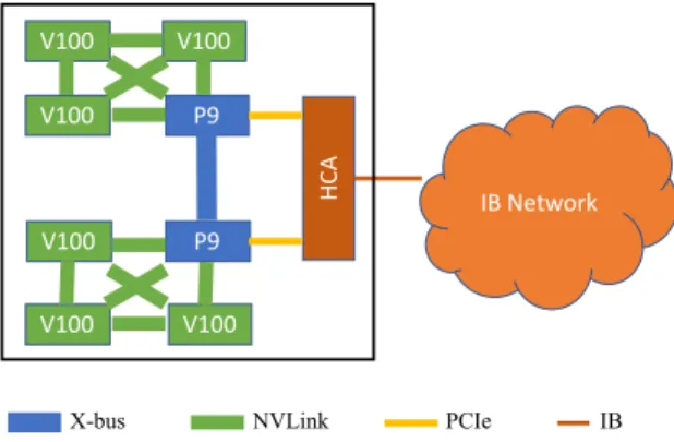
Summit is Oak Ridge National Laboratory’s 200-petaflop supercomputer. It consists of 4,608 com-pute nodes connected to an InfiniBand (IB) network. Specifically, Summit has 256 comcom-puter racks, each of which has 18 compute nodes. A Summit node contains two IBM Power9 (P9) CPUs, six NVIDIA V100 GPUs, and one Mellanox ConnectX-5 Host Channel Adapter (HCA). Fig. 1 shows a simplified block diagram of a single Summit node.
A P9 CPU contains 22 cores and operates at 3.07 GHz. Each P9 core supports up to four hardware threads. It is capable of doing 650 gigaflops of double-precision floating-point arithmetic. In contrast, a single V100 GPU contains 80 streaming multiprocessors and operates at 1.33 GHz. It is capable of doing 7 teraflops of double-precision arithmetic.
A P9 can access its corresponding 256 GB of DDR4 system memory at the peak rate of 170 GB/s. Each V100 can access its 16 GB of high-bandwidth memory at the peak rate of 900 GB/s. Additionally, each node has 1.6TB of non-volatile memory that can be used as a burst buffer.
A P9 is connected to 3 V100s via NVLink at the peak rate of 50 GB/s. The 3 V100s are also connected to each other via NVLink at the same peak rate. This P9 is also connected to the other P9 in the node via IBM’s X-bus at the peak rate of 64 GB/s. Furthermore, it is connected to the HCA in the node at the peak rate of 16 GB/s. The dual-port HCA is responsible for inter-node communication. The dual-rail Mellanox EDR IB network can handle node injection rate of 23 GB/s. Finally, the HCAs in all the nodes and the switches in the IB network form a nonblocking, fat-tree topology of three levels. More details about the system architecture of Summit can be found in [11].
V100 V100 V100 P9 V100 V100 V100 P9 HCA IB Network NVLink X-bus PCIe IB
Figure 1: A simplified block diagram of Summit node without showing the memory components. The thicker the link, the higher the bandwidth.
2.2
Message Passing Interface (MPI)
Message Passing Interface (MPI) is an evolving, open standard driven by the HPC community [5]. It specifies an Application Programming Interface (API) for writing portable programs in message passing parallel programming model [12]. The evolution of the standard has been from MPI-1.0 in 1994 to MPI-3.1 in 2015, and it is still ongoing. MPI is widely used in the HPC community.
Since MPI is just a library interface specification, there exist several well-tested and efficient implementations of MPI. Many of them are open-source, e.g., MPICH [6] and OpenMPI [7]. MPI on Summit is provided by IBM Spectrum MPI, which is based on OpenMPI and fully implements MPI-3.1.
MPI facilitates an evolutionary approach for programming. It is easy to use MPI in an existing program written in C or Fortran. In addition, the programmer can control many details of data communication using MPI. As a result, one can get started fairly quickly with MPI, using just the basics, and come to the more sophisticated tools only when necessary.
MPI supports the programming style of Single Program Multiple Data (SPMD). SPMD achieves parallelism by allowing multiple instances of the same program to operate on different subsets of the data concurrently. For MPI, these instances (called MPI processes) know about each other and can collaborate by exchanging data through messages. An MPI program has the following structure.
#include "mpi.h"
int main (int argc, char *argv[]) { MPI_Init(&argc,&argv); MPI_Comm_size(MPI_COMM_WORLD, &size); MPI_Comm_rank(MPI_COMM_WORLD, &rank); .... MPI_Finalize(); }
An MPI job is created by an initialization call MPI Init and ended by a finalization call MPI Finalize. During initialization, each MPI process is assigned a unique ID called rank. The communicator MPI COMM WORLD is an object describing all the MPI processes that the job starts with, and its size can be queried.
The support for both SPMD-style programming and evolutionary improvements by MPI enhances programmer productivity. Most of the modern HPC applications that run on Summit are written in MPI.
Each MPI process has its own private memory space. The most basic mechanism for creating data objects in that space is to call the malloc function in C. Data is moved from the address space of one process to that of another process through sending and receiving messages. In MPI, the C
functions MPI Send and MPI Recv are used for sending and receiving data messages, respectively. These two functions must be matched to create a correct MPI program. This implements the so-called point-to-point data communication.
Besides providing point-to-point communication interfaces, MPI also provides interfaces for col-lective communication, i.e., communication that involves a group or groups of MPI processes. One C function that receives much attention is MPI Barrier to implement barrier synchronization. This function blocks the caller until all group members have called it.
MPI started with two-sided point-to-point communication and collective communication. Then it extended to include one-sided communication in MPI-2.0 and nonblocking collectives in MPI-3.0.
2.3
OpenSHMEM
OpenSHMEM (Open-standard Symmetric Hierarchical MEMory) provides an alternative to MPI for HPC. It is another evolving, open standard driven by the HPC community [1, 8]. In contrast to MPI, OpenSHMEM specifies an API for writing programs in Partitioned Global Address Space (PGAS) parallel programming model1. An OpenSHMEM program consists of a set of processes,
referred to as Processing Elements (PEs). PGAS assumes a global memory space that is logically partitioned into portions that are local to each PE. The evolution of OpenSHMEM has been from 1.0 in 2012 to 1.4 in 2017 and is still ongoing.
An OpenSHMEM program has the following structure. #include "shmem.h"
int main (void) { shmem_init(); npes = shmem_n_pes(); mype = shmem_my_pe(); .... shmem_finalize(); }
Similar to MPI, OpenSHMEM supports evolutionary, SPMD-style programming for distributed memory systems and thus improves programmer productivity. An OpenSHMEM job is created by an initialization call shmem init and ended by a finalization call shmem finalize. During initialization, each PE is assigned a unique ID called mype. OpenSHMEM provides a mechanism for counting the number of PEs that the job starts with, but there is no concept of a communicator.
The similarity in program structures between MPI and OpenSHMEM lowers the bar to entry for using OpenSHMEM. However, in contrast to MPI’s two-sided send and receive operations, Open-SHMEM provides a one-sided communication model. This communication model enables greater efficiency through lower overheads for algorithms with regular communication like matrix multipli-cation and stencil computation, as illustrated in this paper. It also allows OpenSHMEM to better support irregular algorithms such as graph algorithms and sparse matrix multiplication. In these algorithms, the working set changes during the course of execution, and one-sided communication provides ability to efficiently handle such dynamic communication patterns. Because one-sided com-munication eliminates serialization and matching overheads associated with two-sided messaging, OpenSHMEM can be ideal for unstructured small-size data communication patterns.
OpenSHMEM’s PGAS aims to improve programmer productivity while at the same time aiming for high performance. Programmer productivity is improved by providing a more global view of the HPC algorithms and by the same data referencing semantics of shared memory systems. High performance is achieved by distinguishing between local (cheap) and remote (expensive) memory accesses. The portion of the shared memory space in a PE is affinitized to that PE, thereby exploiting locality of reference. The access to a remote memory space may take advantage of Remote Direct
1According to a recent survey, the current PGAS terminology originates from the work on Split-C, where Culler
Memory Access (RDMA) provided by advanced communication devices such as IB. RDMA allows direct access to remote memory without involving the target.
In each PE, a part of the memory space is shared and the rest is private. The C functions shmem malloc and malloc are used to create shared and private data objects, respectively. Open-SHMEM uses shared data objects as the mechanism for data communication among PEs.
One key feature of OpenSHMEM is that the creation of shared data objects is collective and symmetric across all the PEs in a job. Each PE should participate in the creation by making a call to shmem malloc, and every PE should pass the same value in the size argument for that creation. This symmetric management of the global address space allows a remote address to be simply referenced in terms of a tuple of local address and destination PE. This simplifies the translation of the actual remote address and reduces the translation overhead. This address format is used in shmem get for reading data and in shmem put for writing data in OpenSHMEM. In OpenSHMEM, the special memory region reserved for shared data objects is called the symmetric heap.
Another key feature of OpenSHMEM is that data communication is one-sided in nature. This means that a local PE executing a data transfer routine does not require the participation of the remote PE to complete the routine. This key nature enables OpenSHMEM to provide an easier-to-use one-sided communication interface than MPI.
OpenSHMEM may be used in conjunction with MPI in the same program, but with some limi-tations.
2.4
CUDA
CUDA (Compute Unified Device Architecture), introduced by NVIDIA in 2006, enables software developers to use NVIDIA GPUs for general-purpose computing [2]. It has continued to evolve with the current version being 10.2. A CUDA program has the following structure.
__global__ void func(float *x) {...} int main (void) {
...
func<<<numBlocks, blockSize>>>(x); cudaDeviceSynchronize();
... }
A CUDA kernel is declared by adding the specifier global in front of a function func. The kernel launch is specified by using the <<< >>> syntax called the execution configuration. The execution configuration requires two parameters: the number of thread blocks numBlocks and the number of threads in each block blockSize. These two parameters tell the GPU how many threads will run this CUDA kernel concurrently (i.e., SPMD).
A typical GPU consists of a global memory and multiple Streaming Multiprocessors (SM). The global memory is accessible by all the SMs in the GPU and also CPU. Each SM has many CUDA cores. A thread block is executed by a SM, and it does not migrate. Each thread has an ID that it uses to compute memory addresses and make control decisions.
A thread block consists of one or more 32-thread warps. Warps are used to hide latency. They are queued up for work. If one warp must wait on a memory access, another warp can start executing in its place. As a separate set of registers is allocated for all active threads, there is no need for swapping of registers or states. Thus, this execution model has inherent latency hiding capabilities with minimal scheduling overheads.
3
NVSHMEM
NVSHMEM implements OpenSHMEM for NVIDIA GPU clusters [9, 10]. It provides a PGAS that spans memory across the GPUs in the cluster and also provides an API for fine-grained GPU-GPU data movement and synchronization from within a CUDA kernel. Developed by NVIDIA,
NVSHMEM is still at an early stage. The version we will assess is 0.3.1, released in October 2019, which implements and extends OpenSHMEM-1.4. More information about NVSHMEM can be found in https://developer.nvidia.com/nvshmem.
NVSHMEM is created to address an issue in programming GPU-based extreme-scale systems such as Summit. Currently, a common practice is to use MPI+CUDA for programming. Specifically, the application is split into phases of communication and computation with the computation work offloaded onto GPUs. CPUs coordinate the execution on the GPUs and exchange data using MPI when needed.
This CPU-controlled execution model incurs performance overheads caused by phase transition and limits the scalability of HPC applications. The transition between these phases involves waiting for MPI communication to complete before CUDA kernels can be launched or waiting for CUDA kernels to complete before MPI communication can be initialized.
NVSHMEM offers GPU-initiated communication. Using NVSHMEM, developers can write long running kernels that include both communication and computation, reducing synchronization with the CPU. GPU-initiated communication also avoids the overhead of repeated kernel launches and addresses the under-utilization of the GPU during communication and synchronization, and the under-utilization of the network during computation phases.
NVSHMEM exploits the excellent latency-hiding capability that GPUs have to minimize the performance impact due to GPU-initialized communication. Not only computation and communi-cation can be interleaved, but owing to single-cycle warp scheduling on the GPU, the latency can be hidden not only to local GPU device memory but also to remote GPU memory over a network.
NVSHMEM also improves programmer productivity. Besides SPMD-style programming and incremental improvements, a programmer will not have to rely on a hybrid model to orchestrate and overlap between different phases of the application. Restructuring the application code to overlap independent computation and communication phases makes the application code complex. The benefit of such restructuring diminishes when the problem size per GPU becomes smaller.
3.1
Programming Model
A NVSHMEM program has the following structure. #include "nvshmem.h"
__global__ void func(float *x) {...} int main (void) {
nvshmem_init(); npes = nvshmem_n_pes(); mype = nvshmem_my_pe(); cudaSetDevice(mype); x = nvshmem_malloc(...); .... func<<<numBlocks, blockSize>>>(x); cudaDeviceSynchronize() .... nvshmem_finalize(); }
An NVSHMEM job is created by calling nvshmem init and ended by calling nvshmem finalize. The nv-prefix in NVSHMEM is used to distinguish with OpenSHMEM as NVSHMEM can be used in conjunction with OpenSHMEM. During initialization, each PE must select its GPU (with cudaSetDevice, for example). The PE uses one and only one GPU throughout the lifetime of an NVSHMEM job.
NVSHMEM provides nvshmem malloc to create memory allocation for shared data. Memory allocated using any other method is considered private to the allocating PE and is not accessible by
other PEs. There are also nvshmem get and nvshmem put for memory accesses.
3.2
Extensions to OpenSHMEM
One extension to OpenSHMEM is another form of initialization interface. Besides the nvshmem init function, there is another routine nvshmemx init attr that enables easy porting of MPI and Open-SHMEM programs to NVOpen-SHMEM. Specifically, this routine allows initialization of NVOpen-SHMEM based on an MPI communicator or inside an OpenSHMEM job. This is useful when an application is written to use NVSHMEM within a node and MPI across nodes. An OpenSHMEM program using this extension looks like the following.
#include "mpi.h" #include "nvshmem.h" #include "nvshmemx.h"
int main (int argc, char *argv[]) { MPI_Init(&argc,&argv); MPI_Comm_size(MPI_COMM_WORLD, &size); MPI_Comm_rank(MPI_COMM_WORLD, &rank); cudaSetDevice(rank); nvshmemx_init_attr( SHMEMX_INIT_WITH_MPI_COMM, &attr); npes = nvshmem_n_pes(); mype = nvshmem_my_pe(); .... nvshmem_finalize(); MPI_Finalize(); }
Another extension in NVSHMEM is a new interface nvshmemx collective launch that must be used to launch CUDA kernels on the GPU when the CUDA kernels use NVSHMEM synchronization routines. This is a collective call across the PEs in the NVSHMEM job. It takes the same parameters as a CUDA kernel launch routine. If a CUDA kernel in a PE calls NVSHMEM synchronization routines (such as nvshmem wait, nvshmem barrier, or nvshmem barrier all), then it is required to be launched using this routine. Any CUDA kernel not using NVSHMEM synchronization routines is not required to be launched by this routine.
The routines in NVSHMEM can be classified into three parts: those invoked on the host, those invoked on the GPU, and those invoked on the GPU or host. The two mentioned routines, nvshmemx init attr and nvshmemx collective launch, can only be called from the host in the current version of NVSHMEM. In the current version, runtime initialization and termination, mem-ory management, querying pointers, querying PE information, and collective kernel launch are all only supported from the host.
One-sided remote (atomic) memory access, memory ordering, point-to-point synchronization and collectives are supported from both the host and the GPU. In addition, there are CUDA-specific extensions of remote memory access and collective routines that are supported either only on the host or only on the GPU.
NVSHMEM provides grouped operations, which allow transfers to be more efficient through the participation of full thread blocks or warps. For example, NVSHMEM provides an extension nvshmemx get block for data reads. This new routine is called collectively by every thread in the calling thread block, and with exactly the same arguments. The block and warp extensions enable the NVSHMEM runtime to leverage all the threads in a block or warp to get the data from the destination PE concurrently if the destination GPU of the call is p2p connected. If the destination GPU is connected via InfiniBand, then a single thread in the block can issue an RMA read operation to the destination GPU. Grouped versions of OpenSHMEM collective are also provided and can make
use of multiple threads to perform collective operations, such as parallel reduction operations in case of a collective reduction operation or sending data in parallel.
3.3
Differences from OpenSHMEM
NVSHMEM, 0.3.1 does not yet support all of the OpenSHMEM 1.4 API. Furthermore, NVSHMEM relaxes the memory ordering semantics of OpenSHMEM to allow more efficient implementation on NVIDIA GPUs. We describe these changes.
First, blocking get operations are not guaranteed to be in program order. A blocking get op-eration returns to the destination array at the local PE, after the data has been delivered. The OpenSHMEM specification also implicitly guarantees that any two get operations are always exe-cuted in program order. This ordering of get operations requires the implementation to include an appropriate memory barrier in each get operation, resulting in sub-optimal performance. NVSH-MEM relaxes the ordering requirement of get operations and requires the programmer to use a fence where such ordering is required. The completion semantics of get remain unchanged from the specification. The result of the get is available for any dependent operation that appears after it, in program order.
Second, fence orders blocking get operations. NVSHMEM extends the semantics of shmem fence to order get operations. The shmem fence function does not order non-blocking get operations as specified in the OpenSHMEM specification.
4
Assessment Methodology
In this section, we detail our assessment methodology for each NVSHMEM application we ran on Summit. We used usability, functionality, and scalability as our three assessment criteria.
4.1
Usability
In our assessment, usability pertains specifically to our experiences in the development of a correct NVSHMEM application. We will assess the amount of efforts required to identify and fix bugs in our application. These bugs may occur at compile time or at run time, but they can be corrected by us, the users of NVSHMEM.
Because it is difficult to assess usability in a quantitative yet unbiased manner, we will present our assessment of usability in the form of a list of descriptions about the programming efforts we have made.
4.2
Functionality
In our assessment, functionality refers to the robustness of NVSHMEM itself. Different from usabil-ity, functionality is all about the bugs located inside NVSHMEM. Although NVSHMEM is already open source, it is generally the responsibility of the NVSHMEM implementer, NVIDIA in our case, to locate and correct these bugs.
A major challenge in HPC programming is that usability issues and functionality issues often mingle together. When an application fails to run correctly, the application developer often has a hard time to determine whether the bugs are in the application or in the underlying programming systems.
Functionality is also not easily quantifiable. Therefore, we will present our assessment of func-tionality as a list of descriptions of the debugging efforts we have made.
4.3
Scalability
In our assessment, scalability focuses on how well the total execution time of an NVSHMEM applica-tion scales with the number of allocated compute nodes on Summit (called the node count hereafter for simplicity).
The HPC community generally considers two cases: strong scaling and weak scaling. In the strong-scaling case, the size of the overall problem to be solved is fixed. As a result, the larger the node count, the smaller the problem size per node. In the weak-scaling case, however, the problem size per node is fixed. Therefore, the larger the node count, the larger the overall problem size. We will look into both cases.
Strong scaling relates to the goal of reducing the total execution time by using more computing power. The best scenario is when the parallel efficiency remains 100% regardless of the node count. In our assessment, parallel efficiency is defined as the ratio of the speedup to the node count. Weak scaling, in contrast, is related to the goal of solving larger problems by using more computing power. The best scenario is when the total execution time remains the same regardless of the node count. In our assessment of scalability, these baselines can become helpful.
Another baseline we use is to only consider performance comparison against the 1-node case, not the 1-GPU case. This methodology allows us to solve a larger problem size which can lead to a longer solution time so that its measurement becomes more reliable. The time spent in data initialization and in result checking will not be counted in the total execution time in our assessment. We collect results from three runs for each setting to minimize run-to-run variations.
5
Matrix Multiplication
The first math kernel we used for our assessment of NVSHMEM is matrix multiplication. Specifically, we consider the problem of multiplying two n×n matrices of double-precision floating-point numbers A and B as matrix C. In the following subsections, we will provide details on our NVSHMEM implementation of matrix multiplication as well as our assessment in terms of usability, functionality, and scalability.
5.1
Code Description
To create an NVSHMEM application for matrix multiplication, we did a straightforward porting from a code written in C and OpenSHMEM. The OpenSHMEM code is one of the “textbook” examples provided by the OpenSHMEM community and can be found at https://github.com/ openshmem-org/openshmem-examples/blob/master/C/shmem_matrix.c.
The main data structures in the OpenSHMEM code are three two-dimensional arrays holding the values of matrices A, B, and C. These arrays are distributed among N PEs and allocated in the symmetric heap. The code takes a column-wise data decomposition approach, and each PE will hold several columns of the three matrices.
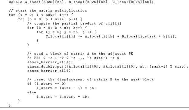
The main control-flow structure (shown in Figure 2) is a nested loop of two-level depth. The outer level iterates over the number of rows n, and the inner level iterates over the number of PEs N . The loop body contains three phases: computing the partial product of C followed by sending a block of A to the adjacent PE followed by updating the displacement of B to the next block.
At a higher level, the OpenSHMEM code iterates over n rows. In each iteration it executes a computation phase followed by a communication phase that performs circular shifts. A circular shift moves the data in each PE to its right neighbor concurrently, as illustrated in Figure 3. After N circular shifts, any PE will be able to see the data stored in all the other PEs. For the matrix-multiplication kernel, it means that each PE will read the whole data in A when all the loop iterations are completed. Each PE multiplies the entire A with its portion of B to derive its portion of C.
5.2
Usability
• We extended the original code to include the case where n is not evenly divisible by N . This extension leads to additional complexity of coding because updating the displacement of B becomes trickier. In such a case, not all the PEs hold data of the same size.
• We corrected a bug in the OpenSHMEM code. Result verification let us realize that this “text-book” example sometimes produces an erroneous answer. It turns out that the implementation
int s i z e ; // n u m b e r of PEs int r a n k ; // my PE id int nb = C O L U M N S / s i z e ; // n u m b e r of c o l u m n s in e a c h PE int i _ s t a r t = r a n k * nb ; // the d i s p l a c e m e n t of m a t r i x B d o u b l e A _ l o c a l [ R O W S ][ nb ] , B _ l o c a l [ R O W S ][ nb ] , C _ l o c a l [ R O W S ][ nb ]; // s t a r t the m a t r i x m u l t i p l i c a t i o n for ( i = 0; i < R O W S ; i ++) { for ( p = 0; p < s i z e ; p ++) { // c o m p u t e the p a r t i a l p r o d u c t of c [ i ][ j ] for ( k = 0; k < nb ; k ++) { for ( j = 0; j < nb ; j ++) { C _ l o c a l [ i ][ j ] += A _ l o c a l [ i ][ k ] * B _ l o c a l [ i _ s t a r t + k ][ j ]; } } // s e n d a b l o c k of m a t r i x A to the a d j a c e n t PE // PE : 0 - > 1 - > 2 - > ... - > size -1 - > 0 s h m e m _ b a r r i e r _ a l l () ; s h m e m _ d o u b l e _ p u t (& A _ l o c a l [ i ][0] , & A _ l o c a l [ i ][0] , nb , ( r a n k +1) % s i z e ) ; s h m e m _ b a r r i e r _ a l l () ; // r e s e t the d i s p l a c e m e n t of m a t r i x B to the n e x t b l o c k if ( i _ s t a r t == 0) i _ s t a r t = ( s i z e - 1) * nb ; e l s e i _ s t a r t = i _ s t a r t - nb ; } }
Figure 2: The pseudo code of matrix multiplication written in OpenSHMEM.
PE0 PE1 PE2 (3,4) (5,6) (7,8) (7,8) (3,4) (5,6) (5,6) (7,8) (3,4) (3,4) (5,6) (7,8) Step 1 Step 2 Step 3
Figure 3: An illustration of circular shift. When this operation is performed N times, the data will be back to its origin.
of circular shifts in the code has a major flaw. Specifically, the implementation uses the same memory address for both the source and the destination when doing remote writes, which can lead to a data race if not synchronized carefully.
To address this issue, our NVSHMEM application stages a circular shift by allocating a buffer for each PE to hold the new value temporarily and then calling for a barrier before copying the new value to where it should be.
5.3
Functionality
For this example, we did not find any issues within NVSHMEM. This is largely due to the fact that we implemented a simple algorithm for matrix multiplication that requires us to use only a handful of basic NVSHMEM routines.
5.4
Scalability
For the assessment of scalability, we ran the kernel for the problem size of 1024×1024 (i.e., n = 1,024) and conducted a strong scaling experiment where we varied the node count from 1 to 128. We did not run the kernel with more than 128 nodes because we wanted to ensure that each PE had some data to work on. If we allocated 256 nodes, for example, then there are 1,536 GPUs and thus 1,536 corresponding PEs. In this case, some of the PEs will not get any data since there are only 1,024 columns to distribute.
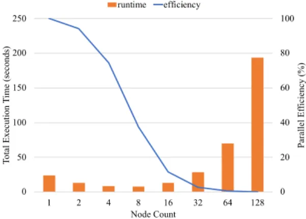
Fig. 4 shows the result of strong scaling. In the figure, the x-axis represents the node count, and the y-axis represents the total execution time (left) as well as the parallel efficiency (right). We make two observations. First, the curve of execution time follows a U pattern. Second, the parallel efficiency drops quickly. As we have discussed in Section 4.3, the best strong scaling occurs when the parallel efficiency is 100%. Clearly, our NVSHMEM application is far from ideal. A better application would have the parallel efficiency drop gradually. So we looked into how to optimize this application. 0 20 40 60 80 100 0 50 100 150 200 250 1 2 4 8 16 32 64 128 P ara ll el E ffi ci enc y (%) Tot al E xe cut ion T im e (s ec onds ) Node Count runtime efficiency
Figure 4: Strong scaling of matrix multiplication.
We looked into the performance of circular shifts, which defines the main communication phase in our application. Fig. 5 provides some insight on how to optimize its behavior. In the figure, the x-axis represents the node count, and the y-axis represents the total execution time on a logarithmic scale. First, we observe that the execution time of circular shifts, the grey bars in the figure, increases with increased node count. Second, this time determines the total execution time of the application when the node count becomes large. As a result, one can improve the performance of the application by spending less time in its communication phase.
One way to reduce the execution time of circular shifts is to shift multiple rows of data at once. We explained in Section 5.2, that the incoming write must be buffered in order to implement
0.1 0.5 2.0 8.0 32.0 128.0 1 2 4 8 16 32 64 128 Tot al E xe cut ion T im e (s ec onds ) Node Count
matmul cshifts (1 row) cshifts (all rows)
Figure 5: The role of circular shifts in matrix multiplication.
circular shifts correctly. This requirement introduces barrier overheads. These barrier overheads become more significant as the node count increases. Therefore, shifting more rows in one remote write should effectively reduce the amount of the barrier overheads. The yellow bars in Fig. 5 confirm that it is indeed the case. These bars represent the resulting execution times when all the rows (i.e., 1,024 in our run) are shifted in one remote write. It is clear that the execution time of circular shifts has been significantly reduced, especially in the case of large node count.
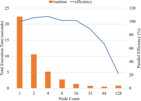
Fig. 6 shows the result of strong scaling after the application is optimized by shifting all the rows at once. The x-axis represents the node count, and the y-axis represents the total execution time (left) as well as the parallel efficiency (right). Similar to the unoptimized version, the curve of execution time still follows a U pattern. However, the smallest execution time occurs at a larger node count; it occurs at 64 nodes instead of 8 nodes. More importantly, the optimized version takes much less time to run and has better strong-scaling behavior.
From this figure, we also notice that the parallel efficiency exceeds 100% when running at small scales. We have not been able to confirm the root cause of this performance anomaly but strongly suspect that the caching effect may play an important role here.
0 20 40 60 80 100 120 0 5 10 15 20 25 1 2 4 8 16 32 64 128 P ara ll el E ffi ci enc y (%) Tot al E xe cut ion T im e (s ec onds ) Node Count runtime efficiency
Figure 6: Strong scaling of optimized matrix multiplication.
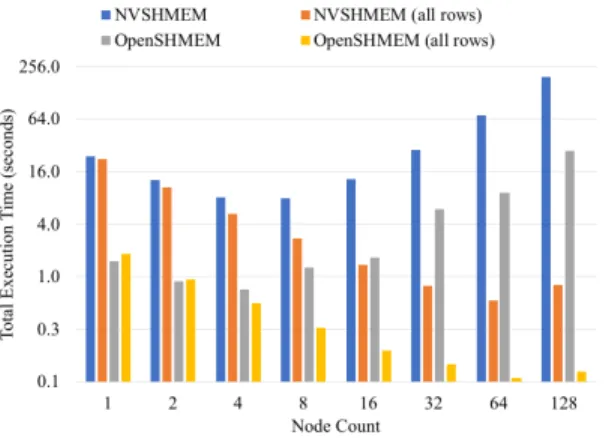
We have also compared the performance of our ported NVSHMEM code against its original OpenSHMEM version. Fig. 7 shows the result of this comparison. In the figure, the x-axis and the y-axis represent the node count and the total execution time in the logarithmic scale, respectively. From the figure we observe that, the unoptimized NVSHMEM version performs the worst in the comparison. However, the optimized NVSHMEM version performs better than the original Open-SHMEM version at large scales. The best version is the OpenOpen-SHMEM version optimized by the same
approach, i.e., shifting all the rows at once in the operation of circular shifts. More importantly, the OpenSHMEM code always performs better than its NVSHMEM counterpart.
Figure 7: Performance comparison to the OpenSHMEM code.
When we reported this comparison result to NVIDIA, they argued that such a comparison cannot render a fair assessment of NVSHMEM. From their viewpoint, NVSHMEM on GPU and OpenSHMEM on CPU are significantly different implementations. In addition, a data set size of 1024×1024 is too small to guarantee the high utilization of GPUs. To address their concern, we have conducted additional experiments evaluating the impact of problem size and work location. We present our findings in the next two subsections.
5.5
The Impact of Problem Size
Our prior experiments show the limited scaling of matrix multiplication in the strong-scaling case. Specifically, the execution time decreases when more compute nodes are used. But the execution time increases when the node count exceeds a certain threshold. In other words, running at the largest system scale may not necessarily lead to the shortest execution time. In the worst case, it may result in the longest running time. Therefore, there comes a question of what limits the scaling, the problem size or the NVSHMEM implementation?
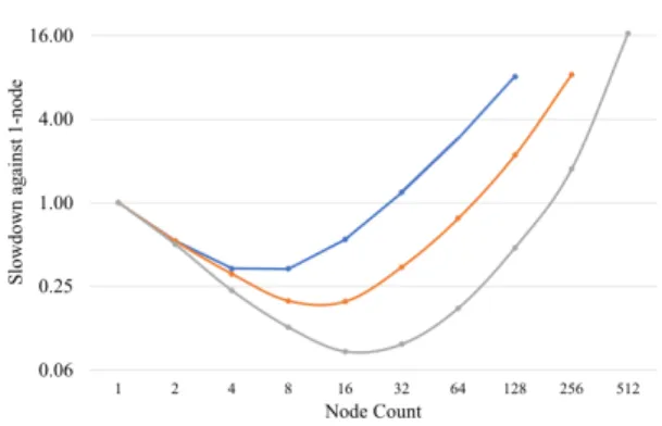
To answer the above question, we conducted a new experiment that measures the execution times at different system scales for a few problem sizes. Figures 8 shows the experimental results. In the figure, the x-axis indicates the number of nodes used. The y-axis represents the ratio of the execution time to the execution time with one single node. Thus, the lower the y-value, the shorter the execution time. In addition, any y-value above 1.0 indicates that the execution is slower than the execution with one node and is therefore undesirable.
What we seek to discover is whether or not a large problem size “moves” the lowest point of the curve to the right? If it does, then we can confirm that the limited strong-scaling is improved when the problem size becomes larger. We find from Figures 8 that it is indeed the case. In other words, when all the compute nodes have enough computational work to do, the increase in communication time due to larger system scale can be masked off.
Finally, we make two additional notes about the results. First, we have not completely answered the question. We have only confirmed that the problem size can influence the strong-scaling behavior. It remains questionable how much the NVSHMEM implementation can influence. Second, we caught a performance issue of NVSHMEM at 512 nodes. The 16-fold slowdown looks very abnormal to us.
5.6
The Impact of Work Location
Our prior experiments show that a SHMEM implementation of matrix multiplication runs faster than its NVSHMEM port, and that creates a concern about the fairness of the comparison from NVIDIA. NVIDIA argues that it is unfair to evaluate NVSHMEM this way because the computational work
Figure 8: The impact of the problem size on strong-scaling for matrix multiplication. The lower the slowdown, the faster the execution and the better.
is done by different types of computing device. They argue that, when evaluating NVSHMEM, the computational work should always be carried out in GPU. Under this restriction, it has been demonstrated that the NVSHMEM approach can perform better than the mainstream CUDA+MPI approach when writing a program.
However, for an end-user whose focus is on minimizing the time-to-solution, binding to a certain type of computing device seems rather artificial. Out of this curiosity, we conducted a new exper-iment with different levels of restriction, distinguished by where the data is located and by where the computation is done.
Our experiment consists of writing and executing seven different implementations of matrix multiplication for the problem size 4096×4096. These implementations are:
1. The initial data and the final data are in GPU. The computation is done by GPU. The communication is by GPU using NVSHMEM (NVSHMEM).
2. The initial data and the final data are in CPU. The computation is done by CPU. The com-munication is done by CPU using MPI (MPI).
3. The initial data and the final data are in CPU. The computation is done by CPU. The com-munication is done by CPU using SHMEM (SHMEM).
4. The initial data and the final data are in GPU. The computation is done by GPU. The communication is done by CPU using MPI (MPI(cuda)).
5. The initial data and the final data are in GPU. The computation is done by GPU. The communication is done by CPU using SHMEM (SHMEM(cuda)).
6. The initial data and the final data are in GPU. The computation is done by CPU. The communication is done by CPU using MPI (MPI(init)).
7. The initial data and the final data are in GPU. The computation is done by CPU. The communication is done by CPU using SHMEM (SHMEM(init)).
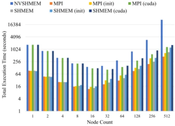
Figure 9 shows the result of this experiment. We first restate what we have observed from prior experiments. We know that NVSHMEM performs better than MPI(cuda) when executing Jacobi solver for the problem size of 32768×32768. We also know that NVSHMEM performs worse than SHMEM when executing matrix multiplication for the problem size of 1024×1024. However, the new experimental result shows that NVSHMEM performs worse than MPI(cuda) when executing matrix multiplication for the problem size of 4096×4096.
The experiment also shows that MPI(init) performs slightly worse than MPI, and the same applies to SHMEM. In other words, if the initial data and the final data must be in GPU, the best
Figure 9: The impact of the restriction level on the performance of matrix multiplication for the problem size of 4096×4096. The lower the execution time the better.
strategy for minimizing the time-to-solution might be using CPU to handle both computation and communication.
Finally, we note that this experiment does not take into account the impact of device-based opti-mizations. In other words, it might be possible that the NVSHMEM code for matrix multiplication can be optimized in such a way that the same optimization cannot be applied to the corresponding SHMEM code. We have already sent the NVSHMEM code to NVIDIA for their CUDA-specific op-timization. Note that the SHMEM code can be optimized as well. For example, in our experiment we only used 6 CPU cores per compute node for the SHMEM code to match with the 6 GPUs in a node. We could have used all the 42 CPU cores per node to execute the SHMEM code.
6
Jacobi Solver
The second math kernel we used for our assessment of NVSHMEM is the Jacobi solver. The Jacobi solver is a popular iterative algorithm for solving a system of linear equations represented as a n × n matrix A. Details of the corresponding NVSHMEM implementation and our assessment follow.
6.1
Code Description
The NVSHMEM implementation of the Jacobi solver was developed by NVIDIA for demonstrating NVSHMEM’s performance benefit. The source code can be found at https://github.com/NVIDIA/ multi-gpu-programming-models/blob/master/nvshmem_opt/jacobi.cu. NVIDIA has provided both unoptimized and optimized versions. For this paper, we assess the optimized version.
The main data structures are two two-dimensional arrays holding the old values and the new values of A. These arrays are distributed among N PEs and allocated in the symmetric heap. The code takes a row-wise data decomposition approach, and each PE holds several rows of the matrices. The main control-flow structure (shown in Figure 10) is an iterative loop of stencil computation and L2-norm calculation. In stencil computation, for each array element, the application computes the average of its north, south, east, and west neighbors. Then it replaces the old value with this computed average. In L2-norm calculation, the application determines whether or not the convergence has reached. The application exits the loop when the convergence check has passed. It also exits the loop when the number of iterations has exceeded a user-provided maximum limit.
There are two major tricks applied to create the optimized version. The first trick is to allow the parallel execution of the two phases. This is achieved by running stencil computation in GPU and L2-norm calculation in CPU. More specifically, stencil computation for the current iteration is performed by the GPU while L2-norm calculation for the previous iteration is performed by the CPU. In addition, the GPU uses NVSHMEM for inter-GPU communication, and the CPU uses MPI
int s i z e ; // n u m b e r of PEs int r a n k ; // my PE id int nb = R O W S / s i z e ; // n u m b e r of r o w s in e a c h PE r e a l A _ l o c a l [ nb + 2 ] [ C O L U M N S ] , A _ l o c a l _ n e w [ nb + 2 ] [ C O L U M N S ]; // s t a r t the J a c o b i s o l v e r w h i l e ( l 2 _ n o r m > tol && i t e r < i t e r _ m a x ) { // p e r f o r m the s t e n c i l c o m p u t a t i o n for ( i = 1; i < nb +1; i ++) { for ( j = 1; j < COLUMNS -1; j ++ ) { n e w _ v a l = 0 . 2 5 * ( A _ l o c a l [ i ][ j + 1] + A _ l o c a l [ i ][ j - 1] + A _ l o c a l [ i + 1][ j ] + A _ l o c a l [ i - 1][ j ]) ; A _ l o c a l _ n e w [ i ][ j ] = n e w _ v a l ; r e s i d u e = n e w _ v a l - A _ l o c a l [ i ][ j ]; l o c a l _ l 2 _ n o r m += r e s i d u e * r e s i d u e ; } } // a p p l y p e r i o d i c b o u n d a r y c o n d i t i o n s // PE : 0 < - 1 < - 2 < - ... < - size -1 < - 0
s h m e m _ d o u b l e _ p u t (& A _ l o c a l _ n e w [ nb +1][0] , & A _ l o c a l _ n e w [1][0] , COLUMNS , ( rank -1+ s i z e ) % s i z e ) ;
// PE : 0 - > 1 - > 2 - > ... - > size -1 - > 0
s h m e m _ d o u b l e _ p u t (& A _ l o c a l _ n e w [0][0] , & A _ l o c a l _ n e w [ nb ][0] , COLUMNS , ( r a n k +1) % s i z e ) ;
// c a l c u l a t e the L2 - n o r m
M P I _ A l l r e d u c e (& l o c a l _ l 2 _ n o r m , & l2_norm , 1 , M P I _ R E A L _ T Y P E , MPI_SUM , M P I _ C O M M _ W O R L D ) ;
l 2 _ n o r m = std : s q r t ( l 2 _ n o r m ) ; std :: s w a p ( A _ l o c a l _ n e w , A _ l o c a l ) ; i t e r ++;
}
for inter-CPU communication. Since the data is mainly in the GPU, additional data transfers from the GPU to the CPU are required for the CPU to be able to make an MPI Allreduce call for the L2-norm calculation.
The second optimization trick is on the exchange of the array elements at the top and bottom rows in each PE, called halo exchange in scientific programming. Instead of making a global barrier call on all the PEs, the optimized version uses a custom implementation of the barrier in which each PE just synchronizes with its neighbor PEs. By reducing the scope of synchronization, the custom barrier has lower overhead and allows the application to run faster.
6.2
Usability
• Users of scaled codes must exercise care that they provide a data set that is big enough for the parallelism expressed by the application, e.g. there must be at least as many rows as PEs. Robust applications could include testing of user inputs to avoid such problems. While NVSHMEM could ignore this condition silently, providing an error or at least a warning, promotes better communication with the user.
• The application contains a flaw that we did not realize until we modified the code. In the assessment of scalability, we attempted to quantify the performance benefit of using a custom barrier for halo exchange. When we replaced the custom barrier with a global barrier, the code hangs. What is even more troublesome is that the code only hangs sometimes. For example, the application ran fine on 256, 512, and 1,024 nodes. However, the code hung always on 128 nodes and sometimes on 32 and 64 nodes. Clearly, this is not an issue related to scale. With NVIDIA’s help, we were able to address this issue. It turns out that the code modified by us ends up with having two barrier all’s executed simultaneously at the end of the major loop. Because OpenSHMEM (and thus NVSHMEM) does not support concurrent global-barrier executions, the behavior is undefined. More importantly, this experience indicates that some flaws are not easily caught by a novice NVSHMEM user.
6.3
Functionality
• The application crashed with a core dump when we ran it on 4,096 nodes, but it worked fine on 2,048 nodes. It took us quite some time to pinpoint the program location at which the error starts. This is because of the lack of the debugging information. We only saw the error message of “errno 3 pid XXXXX bytes read 0” where “errno 3” means “no such process”. We turned on the runtime debug logging in NVSHMEM, but it did not help. It turns out that the crash was caused by an implementation issue in NVSHMEM. Specifically, the amount of node memory required by NVSHMEM exceeded Summit’s 512GB capacity when many PEs are used. NVIDIA has revised their bootstrapped startup routine to reduce the memory requirement from O(N2) to O(N ) in a later release of NVSHMEM, and we are now able to
run up to 4,602 nodes (the full Summit scale) without any problem.
6.4
Scalability
For the assessment of scalability, we ran the kernel for the problem size of 32768×32768 (i.e, n = 32,768) and varied the node count from 1 to 4096. Similar to the case of matrix multiplication, we chose a problem size that is large enough so that every PE will hold some data. When we allocate 4,096 nodes, it leads to 24,576 GPUs that can be used. As a result, each GPU will get at least 1 row to work on.
Fig. 11 shows the result of strong scaling. The x-axis represents the node count, and the y-axis represents the total execution time (left) as well as the parallel efficiency (right). Again, the curve of execution time follows a U pattern.
The U pattern is typical for the strong-scaling behavior of an HPC application. It indicates that the computation time dominates the total execution time when only a few nodes are used. But when
0 20 40 60 80 100 0 4 8 12 16 20 1 2 4 8 16 32 64 128 256 512 1024 2048 4096 P ara ll el E ffi ci enc y (%) Tot al E xe cut ion T im e (s ec onds ) Node Count runtime efficiency
Figure 11: Strong scaling of the Jacobi solver.
many nodes are used, the communication time dominates. For the U pattern, there always exists a sweet spot that minimizes the overall execution time.
From the figure we also observe that the parallel efficiency drops sharply after 16 nodes. This is correlated with the U-pattern in the execution-time curve. Specifically, the U pattern in the execution-time curve leads to the inverse-U pattern in the speedup curve. In other words, the speedup increases until the sweet spot is reached and then decreases. Since the parallel efficiency is a ratio of the speedup to the node count, the inverse-U pattern in speedup leads to smaller speedup and larger node count, thereby significant reduction in parallel efficiency after the sweet spot.
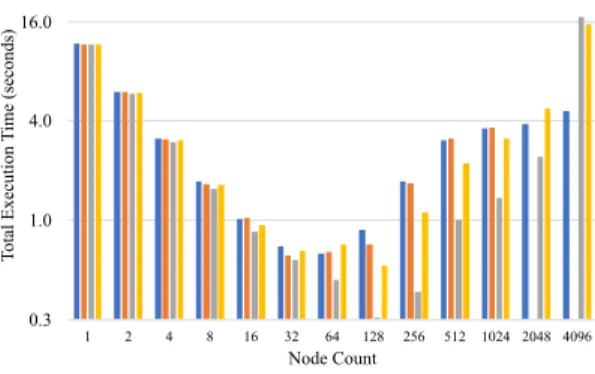
We have increased the problem size to see its impact. Figures 12 shows the results. Similar to the case of matrix multiplication, the limited strong-scaling is improved when the problem size becomes larger. This NVSHMEM application is also far away from the best strong-scaling behavior. Therefore, we looked into how to optimize this already optimized application and will describe our efforts and results in the following paragraphs. We have also caught two robustness issues of NVSHMEM in this experiment. First, the code simply hangs without any error messages when the Jacobi solver code is executed with two nodes for the problem size of 106000×106000. Second, the core dumps when the code is executed for problem sizes larger than 106000×106000. In theory, we should have sufficient memory space to run some of these larger problems. We have reported this issue to NVIDIA and are waiting for their response.
Figure 12: The impact of the problem size on strong-scaling for Jacobi solver. The lower the slowdown, the faster the execution and the better.
Recall that the application has been optimized through the parallel execution of stencil compu-tation (in GPU) and L2-norm calculation (in CPU). This actually is a design choice because both
phases can take turns and be run by GPU. We were interested in determining whether the CPU doing MPI Allreduce causes the performance bottleneck for the entire application and thus modified the code by removing the L2-norm calculation from the application. In other words, the modified application only performs stencil computation and halo exchange in each iteration. Fig. 13 shows the impact on execution time after this modification. The x-axis represents the node count, and the y-axis represents the total execution time in the logarithmic scale. We see that the time spent in the L2-norm calculation is quite significant, but it does not dominate the total execution time.
0.0 0.1 0.5 2.0 8.0 32.0 1 2 4 8 16 32 64 128 256 512 1024 2048 4096 Tot al E xe cut ion T im e (s ec onds ) Node Count NVSHMEM NVSHMEM (no L2 check)
Figure 13: The performance effect by removing the L2-norm calculation.
Fig. 14 shows a performance comparison with three other implementations. The x-axis represents the node count, and the y-axis represents the total execution time in the logarithmic scale. The first alternative implementation, labelled as “MPI”, uses CUDA-aware MPI for inter-GPU communica-tion. The second alternative implementation, labelled as “MPI (overlap)” improves the MPI version by overlapping communication. The third alternative implementation, labelled as “NVSHMEM (global barrier)” de-optimizes the original application by using the global barrier instead. From the figure, we see clearly that the NVSHMEM application performs the best among all the four versions. Its performance advantage gets noticed when the node count becomes large.
0.3 1.0 4.0 16.0 1 2 4 8 16 32 64 128 256 512 1024 2048 4096 Tot al E xe cut ion T im e (s ec onds ) Node Count
MPI MPI (overlap) NVSHMEM NVSHMEM (global barrier)
Figure 14: Performance comparison to other versions.
Note that the missing of the 2,048- and 4,096-node data points for the “MPI (overlap)” imple-mentation is due to the run-time error of invalid configuration argument. This error indicates that the launch of a CUDA kernel fails because some configuration parameters are not set properly. While it is not NVSHMEM’s fault in this case, the experience implies that writing a good NVSHMEM application requires good CUDA expertise and thus decreases the usability of NVSHMEM.
application, we have tested an alternative network configuration for Summit. The default configu-ration minimizes the latency of the network. The new configuconfigu-ration is supposed to maximize the bandwidth. However, the observed performance is quite similar.
Finally, we were able to do a weak-scaling study of the Jacobi solver code. We set the per-node problem size to be 32768×8192, and Fig. 15 shows the result for this setting. Recall that the ideal weak-scaling behavior is when the execution time remains the same no matter how many nodes are used. From the figure it is clear that the NVSHMEM application has nearly ideal weak-scaling behavior, except in the case of 4,096 nodes. We have not been able to identify the root cause of this performance anomaly. 0 4 8 12 16 20 24 28 1 2 4 8 16 32 64 128 256 512 1024 2048 4096 Tot al E xe cut ion T im e (s ec onds ) Node Count
NVSHMEM NVSHMEM (global barrier)
Figure 15: Weak scaling of the Jacobi solver.
7
Horovod
The full application we used for our NVSHMEM assessment is Horovod. Horovod is a very popular deep-learning framework used by many deep-learning applications. In the following we will provide the details of our NVSHMEM implementation of Horovod as well as our assessment results.
7.1
Code Description
Horovod is a framework using which a deep-learning application can be easily written as a Python script. It is an open-source project originally developed by Uber but now extended to become a community-wide effort. Horovod is popular because it only relies on some basic MPI concepts for distributed training, such as size, rank, local rank, and a collective operation called Allreduce. Specifically, the distributed training enabled by Horovod follows the iterative algorithm below:
1. Run multiple copies of the training script, and each script (a) reads a chunk of data, (b) runs it through the model, and (c) computes gradients.
2. Average gradients among all the copies using Allreduce. 3. Update the model.
4. Repeat Step 1.
Note that Step 1 assumes that the model will fit in one MPI rank, and the inter-rank com-munication only occurs in Step 2. More information about Horovod can be found at https: //horovod.readthedocs.io/en/latest/.
To create a NVSHMEM implementation of Horovod, we essentially modified the code responsible for Step 2 above. We ported Horovod in two different ways, resulting in two versions. The two versions differ in the management of NVSHMEM memory space. The first version allocates the
NVSHMEM memory space of the minimally required size at the beginning of each iteration. The second version, in contrast, pre-allocates the NVSHMEM memory space of a sufficiently large size at the beginning of the program execution. This second version is expected to perform better because it reduces the time overheads associates with the dynamic management of the NVSHMEM memory.
7.2
Usability
• The source code of Horovod is relatively complex, so it has taken us quite some time under-standing the code structure. On the other hand, the code is well structured. Thus, porting Horovod to NVSHMEM does not require major modifications to the source code. In our case, we have added three files and modified two files in total to port Horovod to NVSHMEM. • Our porting is rather straightforward. We did not focus on performance optimization. For
such optimization to succeed, a much larger portion of the Horovod source code will have to be modified. For example, NVSHMEM facilitates the fusion of CUDA kernels, but our porting simply replaces Allreduce with the corresponding NVSHMEM host-side API (i.e., nvshmem float sum to all). We also did not take advantage of one-sided communication explicitly nor did we optimize the memory management of Horovod with mostly NVSHMEM memory buffers. Our porting simply copies the data over to the NVSHMEM memory space. • Compiling our NVSHMEM ports is quite challenging. The original Horovod code is compiled
with Gnu C and linked with Gnu C++. Our NVSHMEM ports can be compiled with the same compiler collection, but they will generate run-time errors. We have identified that these errors are caused by the CUDA code (required by NVSHMEM) not being linked properly. It took us quite some time to finally figure out a way to resolve the issue. The fix is rather complex, involving several steps which must set the compiler and linker flags appropriately.
• The design philosophy of Horovod is different from that of NVSHMEM. Horovod initiates its support MPI environment in a lazy fashion. In contrast, NVSHMEM initiates its environment in an eager fashion. This difference has caused an issue of when to initiate NVSHMEM’s envi-ronment. While NVSHMEM provides an API for cloning a given MPI environment, we cannot take advantage of that API. We can only use the most traditional nvshmem init API which requires us to manage MPI processes, NVSHMEM PEs, and CUDA devices very carefully.
7.3
Functionality
We did not confirm any issues from within NVSHMEM.
7.4
Scalability
For the assessment of scalability, we ran a benchmark called tensorflow2 synthetic benchmark.py and collected the performance numbers on Summit for different numbers of nodes. This benchmark is one of Horovod’s out-of-the-box benchmarking support, and it essentially trains the ResNet-50 model on Image Net using Horovod and TensorFlow V2. The performance is measured as the average throughput (i.e., the number of images per second) per GPU. We varied the node count from 1 to 512 with 10 different values. The Horovod version we have measured is V0.19.0.
Figure 16 shows the collected experimental results. From the figure we can see that the through-put performance of the two NVSHMEM ports, nvshmem-v1 and nvshmem-v2, degrades when more nodes are used. However, the slow rate in the reduction of the per-GPU throughput indicates that the two NVSHMEM ports scale reasonably well. Also, the second version performs slightly bet-ter than the first version. This is expected because the first version allocates and deallocates the NVSHMEM memory much more frequently.
In Figure 16 we have also shown the performance numbers of three other versions of Horovod. These versions differ in the implementation of Allreduce. The mpi-mpi version uses MPI for both intra- and inter-node data communication. The nccl-nccl version uses NCCL for both intra- and
Figure 16: Strong scaling of Horovod.
inter-node communication. Finally, the nccl-mpi version uses NCCL for intra-node communication but MPI for inter-node communication. We can see from the figure that our two NVSHMEM ports are superior in performance than the mpi-mpi version but inferior to the other two versions. In other words, NVSHMEM is shown to provide a better alternative to the commonly used CUDA+MPI approach. The exercise of the Jacobi solver has led to the same conclusion, too.
We can make other observations from the figure. First, the three non-NVSHMEM versions have also provided reasonable scalability. Second, the similar performance between the nccl-nccl and nccl-mpi versions seems to imply that the choice of intra-node Allreduce has more weight in determining the overall performance of Horovod than that of inter-node Allreduce. Third, the similar performance between the two NVSHMEM ports indicates that the performance overheads associated with the dynamic allocation of the NVSHMEM memory space is not a significant performance factor.
8
Conclusions
NVSHMEM is an NVIDIA library that implements OpenSHMEM for GPU clusters. In this paper, we presented an assessment of NVSHMEM in terms of usability, functionality, and scalability, by running two math kernels, matrix multiplication and Jacobi solver, and one full application, Horovod, on the Summit supercomputer. The following provides a summary of our experience.
• Writing a correct NVSHMEM application can be non-trivial. The exercise in this paper in-volved not only using NVSHMEM but also porting code to use OpenSHMEM and CUDA. For people not familiar with PGAS models or GPU programming via CUDA, the use of NVSH-MEM may incur a greater learning curve. Debugging NVSHNVSH-MEM codes can be a challenge as well. This is particularly true when the code simply hangs and when bugs only manifest themselves in large-scale runs. In the case of Horovod, the non-coordinated management of MPI processes and NVSHMEM PEs have also created issues. Effective tools for debugging NVSHMEM codes at scale is a good area for future work.
• Writing an efficient NVSHMEM application can also be non-trivial. A straightforward porting from an OpenSHMEM code does not guarantee performance portability, as seen in the case of matrix multiplication. In the case of Jacobi solver, custom barrier is a key to better perfor-mance. For Horovod, a clever management of the host memory, the device memory, and the symmetric heap can be a determining factor. Writing an efficient NVSHMEM application re-quires CUDA expertise to maximize performance. For the current version of NVSHMEM, it is likely that multiple programming tools will be required in order to further improve application performance, adding the complexity in writing a correct program.
• Compiling a NVSHMEM application can be an issue, too. In the case of Horovod, we have seen the challenge of linking CUDA device symbols and NVSHMEM-related libraries. We have
reported this issue to NVIDIA, and their current fix is to require that NVSHMEM and libraries that use NVSHMEM be built as static libraries, not as shared libraries. This limitation makes it difficult to utilize NVSHMEM in an application that takes advantage of shared libraries. • NVSHMEM has performance potential and will improve over time. While it is not the most
efficient at this stage, NVSHMEM has the unique feature of doing all of computation and communication in the GPU which should potentially lead to better performance. When the implementation of NVSHMEM improves over time, we believe that the complexity of program-ming in NVSHMEM will be reduced as well.
• Our exercise of NVSHMEM at scale contributed to making NVSHMEM more robust and preparing it for production release.
9
Acknowledgment
This work is funded by the United States Department of Defense and used the resources of the Oak Ridge Leadership Computing Facility, which is a DOE Office of Science User Facility supported under Contract DE-AC05-00OR22725.
This work was carried out [in part] at Oak Ridge National Laboratory, managed by UT-Battelle, LLC, for the U.S. Department of Energy under contract DE-AC05-00OR22725.
References
[1] B. Chapman, T. Curtis, S. Pophale, S.W. Poole, J. Kuehn, C. Koelbel, and L. Smith. Introduc-ing OpenSHMEM: SHMEM for the PGAS community. In ProceedIntroduc-ings of the Fourth Conference on Partitioned Global Address Space Programming Model, Oct 2010.
[2] CUDA Zone. https://developer.nvidia.com/cuda-zone.
[3] D. E. Culler, A. Dusseau, S. C. Goldstein, A. Krishnamurthy, S. Lumetta, T. von Eicken, and K. Yelick. Parallel programming in Split-C. In Proceedings of the 1993 ACM/IEEE Conference on Supercomputing, Nov 1993.
[4] M. de Wael, S. Marr, B. de Fraine, T. van Cutsem, and W. de Meuter. Partitioned global address space languages. ACM Computing Surveys., 47(4), May 2015.
[5] MPI Forum. https://www.mpi-forum.org. [6] MPICH. https://www.mpich.org.
[7] OpenMPI. https://www.open-mpi.org. [8] OpenSHMEM. http://www.openshmem.org.
[9] S. Potluri, A. Goswami, D. Rossetti, C.J. Newburn, M.G. Venkata, and N. Imam. GPU-centric communication on NVIDIA GPU clusters with Infiniband: A case study with OpenSHMEM. In Proceedings of the IEEE 24th International Conference on High Performance Computing, Dec 2017.
[10] S. Potluri, D. Rossetti, D. Becker, D. Poole, M.G. Venkata, O. Hernandez, P. Shamis, M.G. Lopez, M. Baker, and W. Poole. Exploring OpenSHMEM model to program GPU-based extreme-scale systems. In M.G. Venkata, P. Shamis, N. Imam, and M.G. Lopez, editors, Open-SHMEM and Related Technologies. Experiences, Implementations, and Technologies, pages 18– 35, 2015.
[11] S.S. Vazhkudai, B.R. de Supinski, A.S. Bland, A. Geist, J. Sexton, J. Kahle, C.J. Zimmer, S. Atchley, S. Oral, D.E. Maxwell, and et al. The design, deployment, and evaluation of the CORAL pre-exascale systems. In Proceedings of the International Conference for High Performance Computing, Networking, Storage, and Analysis, Nov 2018.
[12] D.W. Walker. Standards for message-passing in a distributed memory environment. Technical Report TM-12147, Oak Ridge National Laboratory, 1992.