A Classical Catch/Throw Calculus with Tag Abstractions and its Strong Normalizability(Type Theory and its Applications to Computer Systems)

A

Classical

$\mathrm{C}\mathrm{a}\mathrm{t}\mathrm{c}\mathrm{h}/\mathrm{T}\mathrm{h}\mathrm{r}\mathrm{o}\mathrm{W}$

Calculus

with

Tag

Abstractions

and

its

Strong

$\mathrm{N}\mathrm{o}\mathrm{r}\mathrm{m}\mathrm{a}\mathrm{l}\mathrm{i}\mathrm{Z}\mathrm{a}\mathrm{b}\mathrm{i}\mathrm{l}\mathrm{i}\mathrm{t}\mathrm{y}^{\star}$

Yukiyoshi

Kameyama

and

$\mathrm{M}\mathrm{a}s$

ahiko Sato

Department of Information Science,

Kyoto University

{kameyama,

$\mathrm{m}\mathrm{a}\mathrm{s}\mathrm{a}\mathrm{h}\mathrm{i}\mathrm{k}\mathrm{o}\mathrm{I}^{\mathrm{Q}}\mathrm{k}\mathrm{u}\mathrm{i}\mathrm{S}$

.

kyoto-u.

$\mathrm{a}\mathrm{c}$

.

jp

Abstract. The catch and throw constructs

in Common Lisp

provides

a

means

to implement non-local

exits.

Nakano proposed a calculus

$\mathrm{L}_{c/t}$

which has inference rules for the catch and tllrolv constructs, and whose

types

correspond

to

the

intuitionistic

propositional logic. He introduced

the

$\mathrm{t}\mathrm{a}\mathrm{g}-\mathrm{a}\mathrm{b}_{\mathrm{S}}\mathrm{t}\mathrm{r}\mathrm{a}\mathrm{c}\mathrm{t}\mathrm{i}\mathrm{o}\mathrm{n}/\mathrm{a}\mathrm{p}\mathrm{p}\mathrm{l}\mathrm{i}\mathrm{C}\mathrm{a}\mathrm{t}\mathrm{i}\mathrm{o}\mathrm{n}$

mechanism

into

$\llcorner_{\mathrm{c}/t}$

,

which

is

useful to

approximately represent the dynamic

behavior

of tags.

This

paper

examines

the

calculus

$\mathrm{L}\mathrm{K}_{\mathrm{c}/t}$

,

a

classicalized version

of

$\mathrm{L}_{\mathrm{c}/t}$

.

In

$\mathrm{L}\mathrm{K}_{\mathrm{c}/t}$

,

we can write

many

programming

examples

which

are

not

express-ible in

$\llcorner_{c/t}$

, moreover,

algorithmic

contents

can be extracted

from

classi-cal proofs

in

$\mathrm{L}\mathrm{K}_{\mathrm{c}/}\mathrm{t}$

.

We

also prove

several interesting properties

of

$\mathrm{L}\mathrm{K}_{\mathrm{c}/\mathrm{t}}$

including

the strong normalizability.

We

point out

that,

if

we

naively

ap-ply

the well-known reducibility method, the

tag

$\mathrm{a}\mathrm{b}_{\mathrm{S}\mathrm{t}\mathrm{r}\mathrm{a}}\mathrm{C}\mathrm{t}\mathrm{i}_{0}\mathrm{n}/\mathrm{a}\mathrm{p}\mathrm{p}\mathrm{l}\mathrm{i}\mathrm{c}\mathrm{a}\mathrm{t}\mathrm{i}\mathrm{o}\mathrm{n}$

mechanism

is

problematic.

By

introducing

a missing

elimination rule, we

can

successfully

prove

the strong normalizability of

$\mathrm{L}\mathrm{K}_{\mathrm{c}/t}$

.

1

Introduction

The catch and

throw mechanism

in

Common

$\mathrm{L}\mathrm{i}\mathrm{s}\mathrm{p}[15]$

provides a means

to

imple-ment

non-local exits.

The following simple example shows how

to

use

the

catch

and

throw

mechanism in

Common Lisp:

(defun

_multiply

(x)

(catch

_{’zero (multiply2}

$\mathrm{x}$

))

$)$

(defun

_multiply2

(x)

(if (null x)

₁

(if (

$=$

(car x)

$0$

) (throw

’zero

$0$

)

(

$*$

(car x)

(multiply2

(cdr

$\mathrm{x}$

)

$)$

)

$)))$

The

first

function

multiply

sets the catch-point with the

tag

zero and

immedi-ately

calls

the

second

function. The

second one

multiply2

performs the actual

computation

by

recursion.

Given

a

list

of

integers, it calculates

the

multiplica-tion

of the

members in

the

list. If

$0$

is

encountered, then

it

immediately

returns

$0$

without any

further computation. The

$\mathrm{c}\mathrm{a}\mathrm{t}\mathrm{c}\mathrm{h}/\mathrm{t}\mathrm{h}\mathrm{r}\mathrm{o}\mathrm{w}$

mechanism is useful

if

one

wants to

escape from

a

nested

function

call

at

a time.

$\star$

$\mathrm{N}\mathrm{a}\mathrm{k}\mathrm{a}\mathrm{n}\mathrm{o}[8]$

proposed

an

intuitionistic

calculus

with

inference rules which

give

logical

interpretations of the catch and throw constructs.

In

his

calculus

$\mathrm{L}_{c/t}$

,

tags

are

variables

rather than constants, and

a tag

appears freely

in

the

throw-expression,

and

is

bound

in

the catch-expression.

His calculus

ensures

that

no

uncaught

throw

may

occur in a

computation which begins from

a closed

term

(a

term without free tag variables).

An immediate

consequence

of his

representation

is

that,

if

one

wants

to

for-mulate

a logically sound calculus, tag variables

must

have

lexical

scope. However,

tags in Common

Lisp

have

dynamic

scope.

Consequently, the example

above

call-not be

written as a well-formed

term

since

the

tag

zero

in the

throw-expression

is outside of the scope of the

catch-expression.

A

solution

of this problem

is to

$\mathrm{a}\mathrm{b}_{\mathrm{S}}\mathrm{t}\mathrm{r}\mathrm{a}\mathrm{C}\mathrm{t}/\mathrm{a}\mathrm{p}\mathrm{p}\mathrm{l}\mathrm{y}$

the

tag

zero, by which the example

can

be

rewritten as

follows.

(defun

_multiply

(x)

(catch

_’zero

(multiply2

$\mathrm{x}$

’zero))

$)$

(defun

_multiply2

$(\mathrm{X}\mathrm{u})$

(if (null x)

₁

(if (

$=$

(car x)

$0$

) (throw

$\mathrm{u}0$

)

(

$*$

(car x)

(multiply2

(cdr

x)

$\mathrm{u})$

)

$)))$

The function

multiply2

is abstracted

by

the tag variable

$u$

.

When

called,

the

function

is

supplied

an

extra

argument

zero

to

instantiate

the tag

$u$

.

The

key

here

is

that the function

multiply2

no longer

has

free tag variables. It is

$\mathrm{e}\mathrm{a}s$

ily

seen

that the dynamic behavior of tags

in Common

Lisp

can

be

approximately

represented

using

the

$\mathrm{t}\mathrm{a}\mathrm{g}- \mathrm{a}\mathrm{b}\mathrm{s}\mathrm{t}\mathrm{r}\mathrm{a}\mathrm{c}\mathrm{t}\mathrm{i}_{0}\mathrm{n}/\mathrm{a}\mathrm{p}\mathrm{p}\mathrm{l}\mathrm{i}\mathrm{C}\mathrm{a}\mathrm{t}\mathrm{i}_{0}\mathrm{n}$

mechanism.

Although the

$\lambda-$

abstraction

was

used for

$\mathrm{a}\mathrm{b}_{\mathrm{S}}\mathrm{t}\mathrm{r}\mathrm{a}\mathrm{c}\mathrm{t}\mathrm{i}_{1}$

both

_$x$

and

_$u$

in

the example,

the two

variables

differ

in

nature. Therefore,

Nakano

discriminated abstraction

of tag

variables (denoted

as

$\kappa u.t$

)

$\mathrm{f}\mathrm{r}\mathrm{o}\ln$

that of

individual variables

(denoted

as

$\lambda x.t$

).

One possible

defect of

$\mathrm{L}_{c/t}$

is

that

it

has

a

severe restriction on

the

$\lambda-$

introduction rule; all the

$\lambda$

-variables must not

occur

in

the

scope

of any

throw

ex-pression.

For instance, the

term

(catch

$\mathrm{u}$

(lambda

(x) (throw

$\mathrm{u}\mathrm{x})$

))

is

not

a well-typed

$\mathrm{t}\mathrm{e}\mathrm{r}\ln$

in

$\mathrm{L}_{\mathrm{c}/t}$

since

$\mathrm{x}$

appears

in the

body of

the

throw-expression.

Nakano puts

such

a

restriction

to

$\mathrm{L}_{\mathrm{c}/t}$

,

since

he wanted to make the

calculus

intuitionistic.

However,

this

restriction disables one

to

write

practical examples

$\mathrm{w}\mathrm{h}\mathrm{i}_{\mathrm{C}}\mathrm{h}$

uses

the

$\mathrm{c}\mathrm{a}\mathrm{t}\mathrm{c}\mathrm{h}/\mathrm{t}\mathrm{h}_{\Gamma \mathrm{o}\mathrm{w}\mathrm{m}}\mathrm{e}\mathrm{C}\mathrm{h}\mathrm{a}\mathrm{l}\mathrm{l}\mathrm{i}\mathrm{s}\mathrm{m}[5]$

. Moreover,

the

classicalized

$\mathrm{v}\mathrm{e}\mathrm{r}\mathrm{S}\mathrm{i}_{0}11\mathrm{s}$

of the

$\mathrm{c}\mathrm{a}\mathrm{t}\mathrm{c}\mathrm{h}/\mathrm{t}\mathrm{h}\mathrm{r}\mathrm{o}\mathrm{w}$

calculi have

a

possibility

for

$\mathrm{e}\mathrm{x}\mathrm{t}\mathrm{r}\mathrm{a}\mathrm{C}\mathrm{t}\mathrm{i}\mathrm{l}$

algorithmic contents

from

classical

proofs

$[13, 14]$

.

In

this paper,

we

$\mathrm{e}\mathrm{x}\mathrm{a}\mathrm{m}\mathrm{i}_{1}1\mathrm{e}$

a calculus

$\mathrm{L}\mathrm{K}_{c/t}$

,

which

is

essentially

a classicalized

version

of

Naka,

$11\mathrm{O}’ \mathrm{S}$

calculus

$\mathrm{L}_{c/t}$

.

$l\iota^{r}\mathrm{e}$

show that

progralnming

examples

such as

higher-order function with

the

$\mathrm{c}\mathrm{a}\mathrm{t}\mathrm{c}\mathrm{h}/\mathrm{t}\mathrm{h}\mathrm{r}\mathrm{o}\mathrm{W}$

mechanism and

the

classical

encod-ing

of

logical connectives

can

be

written

in

$\mathrm{L}\mathrm{K}_{c/t}$

,

while both

are

not

expressible

in

$\mathrm{L}_{c/t}$

.

We

also prove several

theoretically

interesting

properties of

$\mathrm{L}\mathrm{K}_{c/t}$

,

in

par-ticular, the strong

$11\mathrm{o}\mathrm{r}\mathrm{l}\mathrm{n}\mathrm{a}\mathrm{l}\mathrm{i}_{\mathrm{Z}\mathrm{a}\mathrm{b}\mathrm{i}}1\mathrm{i}\mathrm{t}\mathrm{y}$

“

$\mathrm{a}\iota \mathrm{l}\mathrm{y}$

reduction

sequence

is finite”. This

Standard

ML where tags (exception names) have dynamic

scope

and there

are

$\mathrm{n}\mathrm{o}\mathrm{n}-\mathrm{t}\mathrm{e}\mathrm{r}\iota \mathrm{n}\mathrm{i}\mathrm{n}\mathrm{a}\mathrm{t}\mathrm{i}\mathrm{n}\mathrm{g}$

programs.

The strong normalizability of

$\mathrm{L}_{c/t}$

was

proved

in

[11]

by

a quite elaborate

proof. We simplified the proof in

our

$\mathrm{d}\mathrm{r}\mathrm{a}\mathrm{f}\mathrm{t}[4]$

and

applied it

to

the second author’s

stronger

$\mathrm{c}\mathrm{a}\mathrm{l}\mathrm{c}\mathrm{u}\mathrm{l}\mathrm{u}\mathrm{s}[13]$

,

but

it still needs a

tricky technique,

and

works only for the

calculi

with the

restriction on

the

$\lambda$

-introduction rule.

In this

$\mathrm{p}\mathrm{a}$

.per,

we

develop

a quite natural

proof of the strong normalizability

of the

classical version

$\mathrm{L}\mathrm{K}_{c/t}\mathrm{b}\mathrm{a}s$

ed

on

Tait-Girard’s

reducibility

$\mathrm{m}\mathrm{e}\mathrm{t}\mathrm{h}\mathrm{o}\mathrm{d}[2]$

.

$\mathrm{W}^{\gamma}\mathrm{e}$

analyzed

the failure of earlier proofs, and found

that the reducibility set

for

the

$\mathrm{t}\mathrm{a}\mathrm{g}- \mathrm{a}\mathrm{b}_{\mathrm{S}}\mathrm{t}\mathrm{r}\mathrm{a}\mathrm{C}\mathrm{t}\mathrm{i}\mathrm{o}\mathrm{n}/\mathrm{a}\mathrm{p}\mathrm{p}\mathrm{l}\mathrm{i}\mathrm{C}\mathrm{a}\mathrm{t}\mathrm{i}\mathrm{o}\mathrm{n}$

case

must be

strengthened.

By introducing

a new

language primitive,

we

successfully

define the

reducibility

set which

works

for

proving

the strong normalizability.

The rest

of

this paper is organized as follows:

We

introduce

the

calculus

$\mathrm{L}\mathrm{K}_{c/t}$

and its

extension

$\mathrm{L}\mathrm{K}_{c/t}^{+}$

in

Section

2,

and

give programming

examples in Section

3.

Then

we

turn

our

attention

to the strong normalizability

of

$\mathrm{L}\mathrm{K}_{c/t}^{+}$

.

We

first

explain

the failure of direct application

of reducibility method,

and

then

give

a

proof in Section 4.

Finally,

we

give

concluding

remarks and comparison

to other

works in Section 5.

2

The

calculi

$\mathrm{L}\mathrm{K}_{c/t}$

and

$\mathrm{L}\mathrm{K}_{C}^{+}/t$

This

section

gives

the

calculus

$\mathrm{L}\mathrm{K}_{c/t}$

and its extension

$\mathrm{L}\mathrm{K}_{c/t}^{+}$

.

Before

going

to the

definitions,

we

state several remarks.

The calculus

$\mathrm{L}\mathrm{K}_{c/\mathrm{t}}$

is

esselltially

a

classicalized version

of

Nakano’s

$\mathrm{L}_{\mathrm{c}/t}$

,

so

its definition is almost the

same

as

$\mathrm{L}_{c/\mathrm{t}}$

except that there

is

no

side-condition on

the

$\lambda$

-illtroduction rule. Since

our

calculus can define conjunction

(product type)

and disjunction

(sum type),

we omitted

them

in

$\mathrm{L}\mathrm{K}_{c/t}$

.

The calculus

$\mathrm{L}\mathrm{K}_{c/t}^{+}$

is an

this

paper

can

be written in

$\mathrm{L}\mathrm{K}_{c/t}$

.

2.1

Type Systems

of

$\mathrm{L}\mathrm{K}_{c/t}$

and

$\mathrm{L}\mathrm{K}_{c/t}^{+}$

We

give

the type systems

of

$\mathrm{L}\mathrm{K}_{c/t}$

and

$\mathrm{L}\mathrm{K}_{c/t}^{+}$

, and postpone the reduction rules

to the

next subsection.

First,

we

assume

that there

are

fillitely

many

atomic

types

$\mathrm{B}_{1},$

$\cdots$

,

$\mathrm{B}_{k}$

,

includ-$\mathrm{i}\mathrm{n}\mathrm{g}\perp(\mathrm{f}\mathrm{a}1_{\mathrm{S}}\mathrm{i}\mathrm{t}\mathrm{y})$

.

Definition

1

(Type).

$A::=\mathrm{B}_{1}|\cdots|\mathrm{B}_{k}|Aarrow A|A\triangleleft A$

$\ln$

this

definition,

$arrow \mathrm{i}\mathrm{s}$

the

type

for function space and

$\triangleleft$

is the

type

for

tag-abstraction. The meaning

$\mathrm{o}\mathrm{f}\triangleleft$

will become apparent later.

$14^{\gamma}\mathrm{e}$

use

$A,$

$B,$

$C,$

$\cdots$

for

metavariables

for types. If

a

type does

not

contain

$\mathrm{a}\mathrm{n}\mathrm{d}arrow$

,

then

it is called an

implicational type. We

as

sume

that,

for

each

type

$A$

, there

are

infinitely many

$\mathrm{i}_{11}\mathrm{d}\mathrm{i}\mathrm{v}\mathrm{i}\mathrm{d}\mathrm{u}\mathrm{a}1$

variables

of type

$A$

. We

also

assume

that,

for each implicational type

$A$

,

there

are

infinitely

many

tag

variables

of

type

$A$

.

An important

restriction is

that the types of tag

variables

must be

implicational. Strictly speaking,

$\mathrm{L}\mathrm{K}_{c/t}$

is

not

an extension

of

$\mathrm{L}_{c/t}$

,

since Nakano’s

original calculus

$\mathrm{L}_{c/t}$

does not have this

$\mathrm{r}\mathrm{e}\mathrm{s}\mathrm{t}\mathrm{r}\mathrm{i}\mathrm{C}\mathrm{t}\mathrm{i}_{0}11$

.

However,

we believe that a

tag

variable

of type

$A\triangleleft B$

is

meaningless,

and

that this

restriction is harmless.

At

least,

all the

a,ctual

$\mathrm{c}\mathrm{x}\mathrm{t}\mathrm{l},\mathrm{m}\mathrm{p}\mathrm{l}\mathrm{c}\mathrm{s}$

in

$\mathrm{L}_{\mathrm{c}/t}\mathrm{c}\prime \mathrm{t}\iota 11$

be

$\mathrm{w}\mathrm{r}\mathrm{i}\uparrow[\uparrow,\mathrm{C}]]$

in

$\mathrm{L}\mathrm{K}_{c/t}$

.

We

use metavariables

$x^{A},$

$y^{A},$ $z^{A}$

for

individual

variables and

$u^{A},$ $v^{A},$ $w^{A}$

for

tag

variables.

We

regard

$u^{A}$

and

$u^{B}$

as different

tag

variables

if

$A\not\equiv B$

.

This

implies that

we may sometimes

use

the

same

variable-name

for

different entities

(different types).

Preterms of

$\mathrm{L}\mathrm{K}_{\mathrm{c}/t}^{+}$

are defined as follows.

Definition

2

(Preterm).

$t::=x^{A}|\lambda x^{A}.t|\mathrm{a}\mathrm{p}\mathrm{p}\mathrm{l}\mathrm{y}(t, t)|\mathrm{a}\mathrm{b}\mathrm{o}\mathrm{r}\mathrm{t}(t)$

$|\mathrm{c}\mathrm{a}\mathrm{t}\mathrm{c}\mathrm{h}(u^{A}, t)|\mathrm{t}\mathrm{h}\mathrm{r}\mathrm{o}\mathrm{w}(u^{A},t)|\kappa u^{A}.t|t$

$\bullet$

$u^{A}|t\circ t$

Preterms of

$\mathrm{L}\mathrm{K}_{c/t}$

are those for

$\mathrm{L}\mathrm{K}_{c/t}^{+}$

except

the last

one

$t\circ t$

.

In the

fol-lowing, we sometimes omit the

types

in variables and

preterms,

for example,

throw

$(u, a)B$

is written as

$\mathrm{t}\mathrm{h}\mathrm{r}\mathrm{o}\mathrm{W}(v., a.)$

. Among the

preterms

above,

the

con-structs

catch, throw,

$\kappa$

,

and

$\bullet$

were

$\mathrm{i}_{\mathrm{l}\mathrm{l}\mathrm{t}\mathrm{r}}\mathrm{o}\mathrm{d}\mathrm{u}\mathrm{c}\mathrm{e}\mathrm{d}$

by

Nakano

to represent

the

catch

and

throw mechanism.

Refer to the

following table for the

correspondence

to

similar

constructs

in Common

Lisp and

Standard

$\mathrm{M}\mathrm{L}$

.

$\frac{\mathrm{L}\mathrm{K}_{c/t}/\mathrm{L}\mathrm{K}^{+}\mathrm{C}\mathrm{o}\mathrm{m}\mathrm{m}\mathrm{o}\mathrm{l}1\mathrm{L}\mathrm{i}\mathrm{s}\mathrm{p}\mathrm{s}\mathrm{t}\mathrm{a}11\mathrm{d}\mathrm{a}\mathrm{r}\mathrm{d}\mathrm{n}\iota \mathrm{L}c/t}{\mathrm{c}\mathrm{a}\mathrm{t}\mathrm{c}\mathrm{h}(v.,t)(\mathrm{C}\mathrm{a}\mathrm{t}\mathrm{C}\mathrm{h}\mathrm{u}\mathrm{t})\mathrm{t}\mathrm{h}\mathrm{a}\mathrm{n}\mathrm{d}1\mathrm{e}(\mathrm{u}\mathrm{X})=\succ \mathrm{x}}$

,

$\mathrm{t}\mathrm{h}\mathrm{r}\mathrm{o}\mathrm{W}(u,t)$

(throw

’

$\mathrm{u}\mathrm{t}$

)

raise

$(\mathrm{u}\mathrm{t})$

As noted in the

introduction, tags

in Common

Lisp

(

$\mathrm{e}\mathrm{x}\mathrm{c}\mathrm{e}\mathrm{p}\mathrm{t}\mathrm{i}\prime \mathrm{o}\mathrm{n}$

names

in Standard

$\mathrm{M}\mathrm{L})$

are

represented

as

tag-variables rather

than

collstants.

The preterm

$\kappa u.t$

is

the

tag-abstraction mechanism like

the

$\lambda$

-abstraction

$\lambda x.t$

,

and

the preterm

$t$

$\bullet$

$u$

is

the

tag-application mechanism like

the functional-application

apply

$(t,t)$

.

The

construct

$\circ$

is not

in

Nakano’s

calculus

$\mathrm{L}_{c/t}$

and

is

new

to

this

paper.

$\mathrm{V}^{r}\mathrm{e}$

shall

explain

the role

of this

new

construct

later.

An

individual varia.ble is

bound by the

$\lambda$

-construct,

and a

tag

variable is

bound

by

the

catch-construct

and the

$\kappa$

-construct.

We identify two terms

which

are

equivalent under renaming of bound

$\mathrm{i}\mathrm{n}\mathrm{d}\mathrm{i}\mathrm{v}\mathrm{i}\mathrm{d}\mathrm{u}\mathrm{a}\mathrm{l}/\mathrm{t}\mathrm{a}\mathrm{g}$

variables.

$F\ddagger^{\gamma}(t)$

and

$FTV(t)$

denote

the

set

of free individual variables and the set of free tag variables

in

$t$

,

respectively.

The

type

inference rules of

$\mathrm{L}\mathrm{K}_{c/t}$

and

$\mathrm{L}\mathrm{K}_{c/t}^{+}$

are

given in the natural deduction

style,

and listed in Table 1.

The

inference rules

are

used

to

derive ajudgement

Among the

inference

rules,

the

first four are standard. The rules for

throw

and

catch

reflect

their intended

selnantics,

namely,

$\mathrm{t}\mathrm{h}\mathrm{r}\mathrm{o}\mathrm{W}(u, bB)$

a,borts

the

current

context

so

that

this term

can

be any

type

regardless of the type of

$b$

, and the

type

of

catch

$(uA, a)$

is

the

same

as

$a$

alld

also

the

same as

the type of possibly

thrown terms. The term

$\kappa u^{B}.a$

is a

constructor, alld

it is as

signed

a new

type

$A\triangleleft B$

.

Conversely,

if

$a$

is

of type

$A\triangleleft B$

,

then

applying a

tag variable

$u^{B}$

to

it

generates

a

term of type

$A$

.

$\mathrm{e}\mathrm{l}\mathrm{i}\mathrm{m}\mathrm{i}\mathrm{n}\mathrm{a}\mathrm{t}\mathrm{i}\mathrm{T}\mathrm{h}\mathrm{e}\mathrm{i}\mathrm{n}\mathrm{f}\mathrm{e}\mathrm{r}\mathrm{e}\mathrm{n}\mathrm{c}\mathrm{e}\mathrm{r}\mathrm{u}1\mathrm{e}\mathrm{o}\mathrm{l})\mathrm{r}\mathrm{u}\mathrm{l}\mathrm{e}\mathrm{S}\mathrm{f}\mathrm{o}\mathrm{r}A\triangleleft \mathrm{f}_{0}\mathrm{r}\circ B.\mathrm{S}\mathrm{u}\mathrm{P}\mathrm{p}_{\mathrm{o}\mathrm{S}\mathrm{e}a}\mathrm{h}\mathrm{a}S\mathrm{t}\mathrm{y}(\mathrm{t}\mathrm{h}\mathrm{e}1\mathrm{a}S\mathrm{t}\mathrm{o}\iota 1\mathrm{e})\mathrm{i}\mathrm{s}\mathrm{o}\mathrm{n}1\mathrm{e}\mathrm{p}A\triangleleft B.\mathrm{f}_{\mathrm{f}^{t}\mathrm{w}\mathrm{e}}\mathrm{y}\mathrm{f}_{\mathrm{o}\mathrm{r}}\mathrm{L}\mathrm{K}^{+}$

.

$\mathrm{T}\mathrm{h}\mathrm{i}_{\mathrm{S}}\Gamma \mathrm{u}1\mathrm{e}\mathrm{i}\mathrm{s}c\mathrm{h}\mathrm{a}\mathrm{V}\mathrm{e}\mathrm{a}\mathrm{t}\mathrm{a}\mathrm{g}\mathrm{v}\mathrm{a}\mathrm{r}\mathrm{i}\mathrm{a}\mathrm{k}\mathrm{i}\mathrm{n}\mathrm{d}_{\mathrm{o}\mathrm{f}}\mathrm{a}\mathrm{b}1\mathrm{e}$

$u^{B}$

,

we

can

make a term of type

_$A$

,

namely,

$a$

$\bullet$

$u^{B}$

. However,

even

if

we

have

a

term

$b$

of

type

_$A$

,

we

cannot

make

a

term of type

_$B$

.

In this sense, the type

$A\triangleleft B$

does not have enough

destructors in

$\mathrm{L}_{c/t}$

(and

$\mathrm{L}\mathrm{K}_{c/t}$

), and

as

we shall

show, this

is

the

reason

why

we

cannot directly prove the strong normalizability

of

$\mathrm{L}\mathrm{K}_{c/t}$

. In the

calculus

$\mathrm{L}\mathrm{K}_{c/t}^{+}$

,

we can

partly

achieve

such

construction

when

$B$

is

$B_{1}arrow B_{2}$

.

In that

$\mathrm{C}_{\mathrm{C}}’\mathrm{t}\mathrm{S}\mathrm{e}$

, if

$c$

is

of typc

$B_{1}$

,

then the term

$a.\mathrm{o}c1_{1}\mathrm{a}s$

type

$A\triangleleft B_{2}$

,

which

is smaller

than

the type

$A\triangleleft B$

.

In the

following section,

we shall

explain

how this

“destructor” is

used

in

the proof of

the

strong normalization.

One

should

note

that there

is

$11\mathrm{O}$

side

condition

in

the

$\lambda$

-introduction rule

(the

second rule in Table

2). In

the

intuitionistic

calculus

$\mathrm{L}_{c/t}$

,

a

preterm

$\lambda x^{A}.b$

is

well-typed

only when

$x^{A}$

does not essentially

occur

in

the scope of

any

throw-construct

in

$b^{2}$

.

Let

us

explain the relationship

$\mathrm{b}\mathrm{e}\mathrm{t}_{\mathrm{l}\mathrm{v}\mathrm{e}}\mathrm{e}\mathrm{n}$

the

side-condition

and

the

intuition-istic calculus.

Suppose

$a$

is

a

term of type

$A$

with

$FV(a)=\{x^{B}\}$

and

$FTV(a)=$

$\{u^{E}\}$

.

Then

intuitively

we

have

$Barrow(A\vee E)$

. By

applying the

$\lambda$

-formation

rule

to

$a$

,

we

obtain a

term

$\lambda x^{B}.a$

of type

$Barrow A$

.

Since

$FV(\lambda_{X^{B}}.a)=$

$\{\}$

and

$FTV(\lambda x^{B}.a)=\{u^{E}\}$

, intuitively

we

have

$(Barrow A)\vee E$

.

Hence

we have deduced

2

_{Here we do}

_not

_{give the precise meaning}

_of

_“essential

_{occurrence”}

_in

$\mathrm{L}_{c/t}$

.

Refer

to

[8]

and [11] for details.

$(Barrow A)\vee E$

from

$Barrow(A\vee E)$

.

But

this

is

valid only

in

a classical

calculus,

and

is

not

valid

ill

an

intuitionistic

calculus. Nakano

put

a restriction

on

this

rule to obtain

an

intuitionistic calculus

$\mathrm{L}_{c/t}$

.

As

an

example of type

inference,

the

following

figure is a

proof of the

double-negation-elimination rule.

Here

we abbreviate

$Aarrow\perp \mathrm{a}s\neg A$

.

$\underline{x^{A}\cdot.A}$

$\frac{\frac{\overline{y^{\neg\urcorner}.\neg\neg AA.}\frac{\mathrm{t}.\mathrm{h}\mathrm{r}\mathrm{o}\mathrm{W}(uAAx).1}{\lambda x^{A}\mathrm{t}\mathrm{h}\mathrm{r}\mathrm{o}\mathrm{w}(u^{A},x^{A})\cdot.\cdot\neg A}}{\mathrm{a}\mathrm{p}\mathrm{p}1\mathrm{y}(y,\lambda\urcorner\neg A\mathrm{t}X^{A}.\mathrm{h}\mathrm{r}\mathrm{o}\mathrm{w}(uAAx))\perp}}{\mathrm{a}\mathrm{b}_{\mathrm{o}\mathrm{r}}\mathrm{t}(\mathrm{a}\mathrm{p}\mathrm{p}1\mathrm{y}(y,\lambda x^{A}.\mathrm{t}\mathrm{h}\urcorner\urcorner A\mathrm{w}\mathrm{r}\mathrm{o}(uAX^{A})))\cdot A},,,\cdot.$

.

$\frac{\overline{\mathrm{c}\mathrm{a}\mathrm{t}\mathrm{c}\mathrm{h}(u^{A},\mathrm{a}\mathrm{b}\mathrm{o}\mathrm{r}\mathrm{t}(\mathrm{a}_{\mathrm{P}}\mathrm{P}^{1}\mathrm{y}(y,\lambda_{X^{A}}.\mathrm{t}\mathrm{h}\mathrm{r}\urcorner\urcorner A\mathrm{o}\mathrm{w}(u,X^{A})A))).\cdot A}}{\lambda y^{\urcorner\urcorner}\mathrm{c}\mathrm{a}\mathrm{t}\mathrm{C}\mathrm{h}A.(u^{A},\mathrm{a}\mathrm{b}\mathrm{o}\mathrm{r}\mathrm{t}(\mathrm{a}\mathrm{p}\mathrm{p}1\mathrm{y}(y,\lambda\urcorner\urcorner AA.\mathrm{h}\mathrm{r}\mathrm{o}x\mathrm{t}\mathrm{w}(uAX^{A})))).\neg\neg Aarrow A},\cdot$

Note that,

this

is

a proof

$\mathrm{i}_{1}\mathrm{u}\mathrm{L}\mathrm{K}_{c/}t$

’

but not

a

proof

in

$\mathrm{L}_{c/t}$

,

since in

the application

of the

$\lambda$

-rule

(the

formation

of

$\lambda_{X^{A}.\mathrm{t}\mathrm{h}\mathrm{r}\mathrm{o}}\mathrm{W}(u,$

$x)AA$

),

the abstracted variable

$x^{A}$

occurs

free

in

$\mathrm{t}\mathrm{h}\mathrm{r}\mathrm{o}\mathrm{W}(u^{A}, X)A$

.

The

calculus

$\mathrm{L}\mathrm{K}_{c/t}$

has

no side-condition

on

the

$\lambda$

-rule,

so

the

figure above is a

proof

ill

$\mathrm{L}\mathrm{K}_{c/t}$

(and

$\mathrm{L}\mathrm{K}_{c/t}^{+}$

).

Let

$a,$

$b,$

_$c,$

$\cdots$

be

metavariables for

terlns.

If

$a$

:

$A$

is derived using these

rules,

we write

$\Gamma\vdash a$

:

_$A;\Delta$

where

$\Gamma$

is the

set

of

free,

individual variables

in

$a$

, and

$\Delta$

is

the set of free tag

variables

in

$a.$

For

$\cdot$

example, for the term

$a\equiv \mathrm{t}\mathrm{h}\mathrm{r}\mathrm{o}\mathrm{W}(u^{cAA}, \mathrm{a}_{\mathrm{P}\mathrm{P}^{1}}\mathrm{y}(\mathrm{t}\mathrm{h}\mathrm{r}\mathrm{o}\mathrm{W}(v, x), y^{B}))$

,

we have

_{$\Gamma\vdash a$,}

:

_$D;\Delta$

if

we

put

$\Gamma\equiv\{x^{A}, y^{B}\}$

and

$\Delta\equiv\{v^{C}, v^{A}\}.$

Ill

the

$\mathrm{f}\mathrm{o}\mathrm{l}\mathrm{l}\mathrm{o}\mathrm{W}\mathrm{i}\mathrm{l}\mathrm{l}\mathrm{g}$

,

we shall consider

typable

terms by the type

inference

rules above, and not preterms

in

general.

The calculi

$\mathrm{L}\mathrm{K}_{c/t}$

and

$\mathrm{L}\mathrm{K}_{c/t}^{+}$

correspond to the

classical

propositional

calcu-lus.

We

assume

readers

are familiar

with the Curry-Howard isomorphism; for

instance,

an

implicational type

in

$\mathrm{L}\mathrm{K}_{c/t}$

can

be regarded

as a formula in

logic.

Theorem

3. Let

$A$

be

an

implicational type

in

$\mathrm{L}\mathrm{K}_{c/t}$

(or

$\mathrm{L}\mathrm{K}_{c/t}^{+}$

)

$.$

$A$

is

provable

in the classical

propositional

calculus

_if

and

only

_if

$\emptyset\vdash a$

:

_{$A;\emptyset$}

in

$\mathrm{L}\mathrm{K}_{\mathrm{c}/t}$

for

some term

a.

(Proof Sketch) It

is easy

to

see

that,

$\mathrm{L}\mathrm{K}_{c/t}$

can

prove all the classically valid

theorems

since we

already

gave

the proof of the

law

of

the

double-negation-elimination in

$\mathrm{L}\mathrm{K}_{c/t}$

.

The

inverse

direction

can

be shown

by

an

interpretation

similar

to [13], but details

are

omitted.

$\square$

2.2

Reduction Rules

of

$\mathrm{L}\mathrm{K}_{c/t}$

In

order to

give

the

reduction rules of

$\mathrm{L}\mathrm{K}_{c/t}$

,

we

first state

substitutions.

We

have

three

kinds of

substitutions

in

this

calculus:

$a[b/x^{B}],$

$a[v^{B}/u^{B}]$

,

and

$a[b/*u^{Barrow C}]$

.

The

first

two

$a[b/x^{B}]$

and

$a[v^{B}/u^{B}]$

are usual substitutions. The former

substi-tutes

a term for an individual variable a.nd the latter substitutes a

ta,

$\mathrm{g}$

variable

for

a tag variable. Note

that

$a[b/x^{B}]$

is defined only when

$b$

has

type

_$B$

.

defined

as

usual. The third form

$a[b/*u^{Barrow C}]$

is used for the reduction of the

newly

introduced constructor

$0$

,

and it

is defined in

the

next subsection.

The notion of

1-step

reduction in

$\mathrm{L}\mathrm{K}_{c/t}$

is the

same as

those

defined

by

Nakano,

and

is defined as

the compatible

closure

of the

reduction rules given in

Table

2. Namely, for any

term-context

$C[]$

,

we

have

$C[a.]arrow,1C[b]$

if and

only if

$aarrow 1b$

.

For instance,

we

have the following

reductions:

catch

$(u, \mathrm{a}\mathrm{p}\mathrm{p}\mathrm{l}\mathrm{y}(\mathrm{t}\mathrm{h}\mathrm{r}\mathrm{o}\mathrm{W}(u, x), y))arrow 1\mathrm{c}\mathrm{a}\mathrm{t}\mathrm{c}\mathrm{h}(u, \mathrm{t}\mathrm{h}\mathrm{r}\mathrm{o}\mathrm{W}(u, x))-1x$

$(\kappa v.\mathrm{a}\mathrm{p}\mathrm{p}\mathrm{l}\mathrm{y}(\mathrm{t}\mathrm{h}\mathrm{r}\mathrm{o}\mathrm{W}(v, a),$

$b))$

$\bullet$

$u-1\mathrm{a}\mathrm{p}\mathrm{p}\mathrm{l}\mathrm{y}(\mathrm{t}\mathrm{h}\mathrm{r}\mathrm{o}\mathrm{w}(u, a),$

$b)-1\mathrm{t}\mathrm{h}\mathrm{r}\mathrm{o}\mathrm{W}(u, a)$

Instead

of

having a

one-step

reduction like

catch

$(u, a[\mathrm{t}\mathrm{h}\mathrm{r}\mathrm{o}\mathrm{W}(u, b)/x])-1b$

, the

$\mathrm{c}\mathrm{a}\mathrm{t}\mathrm{c}\mathrm{h}/\mathrm{t}\mathrm{h}\mathrm{r}\mathrm{o}\mathrm{w}$

mechanism

splits

into

two steps

as follows:

catch

$(u, a[\mathrm{t}\mathrm{h}\mathrm{r}\mathrm{o}\mathrm{W}(u, b)/x])-1\mathrm{c}\mathrm{a}\mathrm{t}\mathrm{c}\mathrm{h}(u, (\mathrm{t}\mathrm{h}\mathrm{r}\mathrm{o}\mathrm{W}(u, b)))arrow 1b$

Since

we

did

llot

restrict

any evaluation strategy,

the

reduction in

$\mathrm{L}\mathrm{K}_{c/t}$

is

non-deterministic,

moreover

it

is

not Church-Rosser.

For instance,

the following

term

reduces

to

both

$x^{A}$

and

$y^{A}$

:

catch

$(u, \mathrm{a}\mathrm{p}\mathrm{p}\mathrm{l}\mathrm{y}(A\mathrm{t}\mathrm{h}\mathrm{r}\mathrm{o}\mathrm{w}(u^{A}, X^{A}), \mathrm{t}\mathrm{h}\mathrm{r}\mathrm{o}\mathrm{w}(u^{A}, y^{A})))$

We

do not

think

that

this is

a

defect

of

$\mathrm{L}\mathrm{K}_{c/t}$

because (1)

as

far

as

the strong

$\mathrm{n}\mathrm{o}\mathrm{r}\iota \mathrm{n}\mathrm{a}.\mathrm{l}\mathrm{i}\mathrm{Z}\mathrm{a}\mathrm{b}\mathrm{i}\mathrm{l}\mathrm{i}\mathrm{t}\mathrm{y}$

is

concerned,

it

is preferable to have

as

strong

reduction rules

as

possible,

and

(2)

classical

logic

is said

to

be inherently

$\mathrm{n}\mathrm{o}\mathrm{n}-\mathrm{d}\mathrm{e}\mathrm{t}\mathrm{e}\Gamma \mathrm{m}\mathrm{i}_{1}1\mathrm{i}\mathrm{s}\mathrm{t}\mathrm{i}\mathrm{c}$

.

In

order to

express all possible computations in classical

proofs,

our calculus should

be

non-deterministic.

Later

we

can

choose

one answer

by

fixing

an evaluation

strategy. In

fact,

the second author showed in

[14]

that Murthy’s

$\mathrm{e}\mathrm{x}\mathrm{a}\mathrm{m}_{\mathrm{P}^{\mathrm{l}\mathrm{e}}}[7]$

can

be expressed

in a

$\mathrm{c}\mathrm{a}\mathrm{t}\mathrm{c}\mathrm{h}/\mathrm{t}\mathrm{h}\mathrm{r}\mathrm{o}\mathrm{w}$

calculus.

We may obtain

a various

confluent calculus as a subcalculus of

$\mathrm{L}\mathrm{K}_{\mathrm{c}/t}$

by

restricting reduction rules. Our results

(Subject

Reduction and

Strong

Normal-ization) hold for any properly formulated subcalculus

of

$\mathrm{L}\mathrm{K}_{c/t}$

.

2.3

Reduction Rules of

$\mathrm{L}\mathrm{K}_{c/t}^{+}$

Defining

the

notion

of 1-step

reduction

in

$\mathrm{L}\mathrm{K}_{c/t}^{+}$

is

relatively

more

difficult

than

in

$\mathrm{L}\mathrm{K}_{c/t}$

.

We

first

define

the third form of

substitution

$a[b/*u^{Barrow}]C$

which was left

undefined. This substitution is close

to

one

in Parigot’s

$\lambda\mu- \mathrm{c}\mathrm{a}\mathrm{l}\mathrm{c}\mathrm{u}\mathrm{l}\mathrm{u}\mathrm{S}[12]$

.

It

is

de-fined only when

$b$

has type

$B$

.

Intuitively,

$a[b^{B}/*u^{B-C}]$

replaces

all

the

subterms

in

the form

throw

$(uB-c, c)$

_where

$u^{Barrow C}$

is

free

in

_$a$

,

by

throw

$(u^{C}, \mathrm{a}_{\mathrm{P}\mathrm{p}1}\mathrm{y}(c, b))$

.

For

brevity,

we

use

the

same name

$u$

for the

tag

variable after the substitution

even if

its

type

is changed

(note

that

$u^{Barrow C}$

and

$u^{C}$

are

different tag

variables).

The

precise definition given

below

is

more

complex than this

intuitive

explana-tion

because free

tag variables may appear also in

$c$

$\bullet$

$u$

.

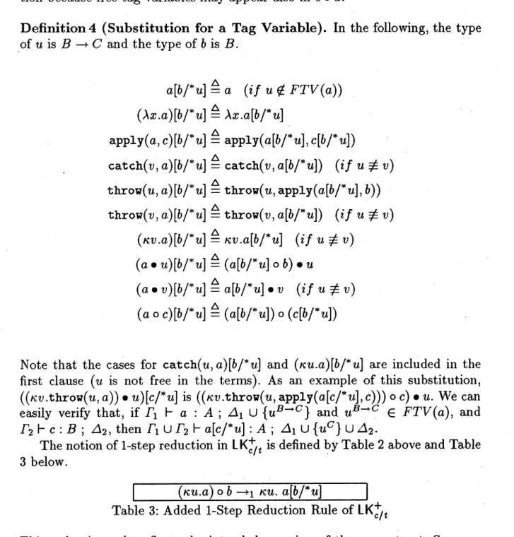
Definition

4 (Substitution for

a

Tag

Variable).

In the following,

the type

of

$u$

is

$Barrow C$

and the type of

$b$

is

$B$

.

$a[b/^{*}u]=\Delta a$

_{$(ifu\not\in FTV(a))$}

$(\lambda X.a)[b/*]u=\Delta\lambda x.a[b/^{*}u]$

apply

$(a, c)[b/*]u=\triangle \mathrm{a}\mathrm{p}\mathrm{p}\mathrm{l}\mathrm{y}(a[b/*u], C[b/*]u)$

catch

$(v, a)[b/*u]=\triangle \mathrm{c}\mathrm{a}\mathrm{t}\mathrm{c}\mathrm{h}(v, a[b/*]u)$

(if

_{$u\not\equiv v$}

)

$\mathrm{t}\mathrm{h}\mathrm{r}\mathrm{o}\mathrm{W}(u, a)[b/*u]=\triangle \mathrm{t}\mathrm{h}\mathrm{r}\mathrm{o}\mathrm{W}(u, \mathrm{a}\mathrm{p}\mathrm{P}\mathrm{l}\mathrm{y}(a[b/*]u, b))$

$\mathrm{t}\mathrm{h}\mathrm{r}\mathrm{o}\mathrm{W}(v, a)[b/*u]=\triangle \mathrm{t}\mathrm{h}\mathrm{r}\mathrm{o}\mathrm{W}(v, a[b/*]u)$

(if

$u\not\equiv v$

)

$(\kappa v.a.)[b/*]u=\triangle\kappa v.a[b/*u]$

_{$(ifu\not\equiv v)$}

$(a \bullet u)[b/*v‘]=\triangle(a[b/*u]\circ b)$

$\bullet$

_$u$

$(a \bullet v)[b/*u]=\triangle a[b/*u]$

$\bullet$

$v$

(if

$u\not\equiv v$

)

(a

$\mathrm{o}c$

)

$[b/^{*}v.]=\triangle(a[b/*u])\circ(c[b/*u])$

Note that the

cases

for

catch

$(u, a)[b/*v.]$

and

$(\kappa u.a)[b/*.u]$

are included in

the

first clause

(

$u$

is

not

free in the

terms). As

an

example of this substitution,

$((\kappa v.\mathrm{t}\mathrm{h}\mathrm{r}\mathrm{o}\mathrm{W}(u, a))$

$\bullet$

_$u$

)

$[c/*u]$

is

$((\kappa v.\mathrm{t}\mathrm{h}\mathrm{r}\mathrm{o}\mathrm{w}(u, \mathrm{a}\mathrm{p}\mathrm{p}\mathrm{l}\mathrm{y}(\mathit{0},[C/*v.], c)))\circ C)$

$\bullet$

$u$

.

We

can

$\mathrm{e}\mathrm{a}s$

ily verify that, if

$\Gamma_{1}\vdash a$

:

$A$

;

$\Delta_{1}\cup\{u^{Barrow C}\}$

and

$u^{Barrow C}\in FTV(a)$

,

and

$\Gamma_{2}\vdash c:B$

;

$\Delta_{2}$

,

then

$\Gamma_{1}\cup\Gamma_{2}\vdash a[c/*u]:A;\Delta_{1}\cup\{u^{C}\}\cup\Delta_{2}$

.

The notion

of 1-step

reduction in

$\mathrm{L}\mathrm{K}_{c/t}^{+}$

is defined

by

Table 2 above

and

Table

3 below.

Table 3: Added

1-Step

Reduction Rule of

$\mathrm{L}\mathrm{K}_{c/t}^{+}$

This

reduction rule reflects

the

intended meaning of the

$\circ$

-construct.

Suppose

is

of type

$A\triangleleft C$

and

it reduces

to

$\kappa u^{C}.a[b/*u]$

where

$b$

is

applied to

all the

throw-expressions

in

$a$

whose

tag

is

$u$

.

We

use the following

abbreviations:

apply

$(\ldots \mathrm{a}\mathrm{P}\mathrm{p}\mathrm{l}\mathrm{y}(b, d_{1})\ldots,$

$dn)$

as

apply

$(b,\overline{d_{1,\ldots,n}d})$

$(... (b\circ d_{1})\ldots)\circ d_{n}$

as

$b\mathrm{o}\overline{d_{1},\ldots,d_{n}}$

\‘A

successive substitution in

the form

$(\cdots(a,[b_{1}/*u])\cdots)[b_{n}/*u]$

is

abbrevi-ated

as

$a[b_{1}, \cdots, b_{n}/*u]$

.

In the

following

we

shall

use

this form of substitution

only

when

$b_{i}$

does

not

contain

$u$

free. We

shall

also

use

a

mixed

simultaneous

substitution

such

as

$[b_{1/,/1}X_{1}, ’\cdot\cdot, \overline{c_{1}1\ldots,C^{k}1}*u, , ..]$

in

the

following.

We

define

$aarrow b$

(zero

or more

step reduction), and

_$aarrow+b$

(one

or more

step

reduction)

as usual.

Then

we

have the subject

reduction

theorem

for

$\mathrm{L}\mathrm{K}_{c/t}$

and

$\mathrm{L}\mathrm{K}_{c/t}^{+}$

.

Theorem

5

(Subject

Reduction).

In

either

$\mathrm{L}\mathrm{K}_{c/t}$

or

$\mathrm{L}\mathrm{K}_{c/t}^{+}$

,

if

$\Gamma\vdash a:A$

;

$\Delta$

and

$aarrow b_{f}$

then

$\Gamma’\vdash b:A;\Delta’$

for

some

$\Gamma’\subset\Gamma$

and

$\Delta’\subset\Delta$

.

Proof.

It

is

an

easy

exercise

by

induction

on

the

length

of the reduction.

Here,

we

verify only the

case

$(\kappa u.a)\mathrm{o}barrow 1\kappa u.a[b/*u]$

. Suppose

$(\kappa u.a)\mathrm{o}b$

is

a

well-typed

term.

Then,

we

have

$\Gamma_{1}\vdash\kappa u.a$

:

$A\triangleleft(Barrow C);\Delta_{1}$

and

$\Gamma_{2}\vdash b$

:

$B;\Delta_{2}$

for

some

$\Gamma_{1},$

$\Gamma_{2},$

$\Delta_{1},$

$\Delta_{2}$

. The first

clause

implies that

_{$\Gamma_{1}\vdash a:A;\Delta_{1}\cup$}

$\{u^{Barrow C}\}$

.

Then

we

have

$\Gamma_{1}\cup\Gamma_{2}\vdash a[b/.*u]$

:

$A$

;

$\Delta_{1}\cup\{v^{C},\}\cup\Delta_{2}$

.

It

follows

that

$\Gamma_{1}\cup\Gamma 2\vdash\kappa u.a.[b/*u]$

:

$A\triangleleft c;\Delta_{1}\cup\Delta 2$

.

$\square$

3

$\mathrm{P}_{\Gamma \mathrm{o}\mathrm{r}\mathrm{a}\mathrm{n}}\mathrm{g}\mathrm{n}\mathrm{n}\mathrm{l}\mathrm{j}\mathrm{n}\mathrm{g}\mathrm{E}\mathrm{x}\mathrm{a}\mathrm{n}\prime 1\mathrm{P}^{1}\mathrm{e}\mathrm{S}$

in

$\mathrm{L}\mathrm{K}_{c/t}$

This

section

shows the

expressiveness

of

$\mathrm{L}\mathrm{K}_{c/t}$

.

The

first

examples

are

Griffin’s

classical

$\mathrm{e}\mathrm{n}\mathrm{c}\mathrm{o}\mathrm{d}\mathrm{i}_{1\mathrm{l}}\mathrm{g}$

of

logical

connectives

such

as conjunction

and

disjunction.

$A$

A

$B\equiv\neg(Aarrow\neg B)$

pair

$(a^{AB}, b)\equiv\lambda x^{Aarrow_{\urcorner}B}.\mathrm{a}_{\mathrm{P}}\mathrm{P}\mathrm{l}\mathrm{y}(\mathrm{a}\mathrm{p}\mathrm{p}\mathrm{l}\mathrm{y}(X, a),$

_$b)$

car

$(c^{A\wedge})B\equiv \mathrm{c}\mathrm{a}\mathrm{t}\mathrm{c}\mathrm{h}(v\cdot, \mathrm{a}\mathrm{b}\mathrm{o}\mathrm{r}\mathrm{t}(A\mathrm{y}\mathrm{a}\mathrm{p}\mathrm{P}^{1}(c, \lambda X\lambda y\mathrm{t}\mathrm{h}\mathrm{r}\mathrm{o}\mathrm{W}A.B.(u^{A}, x))))$

$\mathrm{c}\mathrm{d}\mathrm{r}(cA\wedge B)\equiv \mathrm{c}\mathrm{a}\mathrm{t}\mathrm{c}\mathrm{h}(v^{B}, \mathrm{a}\mathrm{b}\mathrm{o}\mathrm{r}\mathrm{t}(\mathrm{a}\mathrm{P}\mathrm{p}\mathrm{l}\mathrm{y}(C, \lambda_{X^{A}}.\lambda y^{B}.\mathrm{t}\mathrm{h}\mathrm{r}\mathrm{o}\mathrm{W}(v, yB))))$

$A\vee B\equiv\neg Aarrow\neg\neg B$

$\mathrm{i}\mathrm{n}1(a^{A})\equiv\lambda X^{\urcorner}\lambda A.\mathrm{l}y^{\neg B}.\mathrm{a}\mathrm{p}\mathrm{p}\mathrm{y}(x, a)$

$\mathrm{i}\mathrm{n}\mathrm{r}(b^{B})\equiv\lambda x^{\urcorner}\lambda A.\urcorner B.(y\mathrm{a}\mathrm{P}\mathrm{p}\mathrm{l}\mathrm{y}y, b)$

cas

$\mathrm{e}(a^{A};xb^{C}\vee BA.C^{C}; y^{B}.)\equiv \mathrm{c}\mathrm{a}\mathrm{t}\mathrm{c}\mathrm{h}$

(

$u^{c}$

, abort

(apply

$(a,\overline{d,e})$

))

$d\equiv\lambda x^{A}.\mathrm{t}\mathrm{h}\mathrm{r}\mathrm{o}\mathrm{w}(u, bC)$

As expected,

we

have

car

$(\mathrm{P}\mathrm{a}\mathrm{i}\mathrm{r}(a, b))arrow a$

and

$\mathrm{c}\mathrm{d}\mathrm{r}(\mathrm{p}\mathrm{a}\mathrm{i}\mathrm{r}(a, b))arrow b$

. Similarly,

we

have case

$(\mathrm{i}\mathrm{n}\mathrm{l}(a);X.b;y.c)arrow b[a/x]$

and

case

$(\mathrm{i}\mathrm{n}\mathrm{r}(a);X.b;y.c)arrow c[a/y]$

.

The

second

$\mathrm{e}\mathrm{x}\dot{\mathrm{a}}\mathrm{m}\mathrm{P}\mathrm{l}\mathrm{e}$

taken

from the

first

author’s

previous

$\mathrm{w}\mathrm{o}\mathrm{r}\mathrm{k}[5]$

uses

the

$\mathrm{c}\mathrm{a}\mathrm{t}\mathrm{c}\mathrm{h}/\mathrm{t}\mathrm{h}\mathrm{r}\mathrm{o}\mathrm{w}$

mechanism in a higher-order function. The function

sqrt-sum

cal-culates,

given a list

of

integers,

the

sum

of square root

of

each

element.

If

there is

a

negative

number

in

the list,

it

immediately stops the

computation and returns

the

number. The program is written in

Common Lisp

like this:

(defun

_sqrt-sum

(x)

(catch

_’negative

(sqrt-sum2

$\mathrm{x}$

))

$)$

(defun

_sqrt-sum2

(x)

(if (null x)

$0$

(if (

$<$

(car x)

$0$

) (throw

’negative

(car

$\mathrm{x})$

)

(

$+$

(sqrt

(car

$\mathrm{x}$

))

(sqrt-sum2

(cdr

$\mathrm{x}))$

)

$)))$

This

program

is

written in

$\mathrm{L}\mathrm{K}_{\mathrm{c}/t}$

,

assuming

that

$\mathrm{L}\mathrm{K}_{c/t}$

is

extended to have

inte-gers, lists

and

so on.

sqrt-sum

$=\Delta\lambda_{X.\mathrm{C}}\mathrm{a}\mathrm{t}\mathrm{C}\mathrm{h}(u, \mathrm{a}_{\mathrm{P}}\mathrm{p}\mathrm{l}\mathrm{y}(\mathrm{s}\mathrm{q}\mathrm{r}\mathrm{t}-\mathrm{s}\mathrm{u}\mathrm{m}2, X) \bullet v\cdot)$

sqrt-sum2

$=\triangle\lambda_{X.\kappa u.\mathrm{R}\mathrm{e}\mathrm{C}}(f, 0, x)$

$f=\triangle\lambda yzw$

.

(if

$(<y0)$

(throw

_{$uy)(\dotplus$}

(sqrt

$y)w)$

)

where

$\mathrm{R}\mathrm{e}\mathrm{c}$

is

the

recursor

on

the

list

type

which

has the

following reduction rules:

$\mathrm{R}\mathrm{e}\mathrm{c}(f, O, nil)arrow,$

_$1a$

$\mathrm{R}\mathrm{e}\mathrm{c}(f, a_{\mathit{3}}ConS(b, c))arrow 1\mathrm{a}\mathrm{p}\mathrm{p}\mathrm{l}\mathrm{y}(\mathrm{a}\mathrm{p}\mathrm{p}\mathrm{l}\mathrm{y}(\mathrm{a}_{\mathrm{P}}\mathrm{p}\mathrm{l}\mathrm{y}(f, b),$

$C),$

$\mathrm{R}\mathrm{e}\mathrm{C}(f, a, c))$

We need the

$\mathrm{c}\mathrm{a}\mathrm{t}\mathrm{c}\mathrm{h}/\mathrm{t}\mathrm{h}\mathrm{r}\mathrm{o}\mathrm{w}$

mechanism through

the

$\lambda$

-abstraction. Again

this

ex-ample cannot be

written in

$\mathrm{L}_{c/t}$

.

4

Strong Normalizability

Ill this section,

we prove

the strong normalizability of

$\mathrm{L}\mathrm{K}_{c/t}$

and

$\mathrm{L}\mathrm{K}^{+}c/t$

.

4.1

Tait-Girard’s reducibility method

Tait-Girard’s

reducibility

$\mathrm{m}\mathrm{e}\mathrm{t}\mathrm{h}\mathrm{o}\mathrm{d}[2]$

is

a

standard technique

to

prove the strong

normalizability

of typed lambda

calculi.

We

first

give an overview

of the

method.

1.

Define

the set of

terlns

Red

$(A)$

for each type

$A$

.

This is by

induction on

the

type.

$a\in \mathrm{R}\mathrm{e}\mathrm{d}(A)=\triangle$

$a$

is

strongly normalizing (if

$A$

is

atomic),

$a\in \mathrm{R}\mathrm{e}\mathrm{d}(Aarrow B)=\triangle \mathrm{a}\mathrm{p}\mathrm{p}\mathrm{l}\mathrm{y}(a, b)\in \mathrm{R}\mathrm{e}\mathrm{d}(B)$

for

any

$b\in \mathrm{R}\mathrm{e}\mathrm{d}(A)$

.

2. Prove three conditions called (CR-1), (CR-2), and (CR-3).

(CR-1)

If

$a\in \mathrm{R}\mathrm{e}\mathrm{d}(A)$

,

then

$a$

is strongly

normalizing.

(CR-2)

If

$a\in \mathrm{R}\mathrm{e}\mathrm{d}(A)$

and

$aarrow 1b$

,

then

$b\in \mathrm{R}\mathrm{e}\mathrm{d}(A)$

.

(CR-3)

If

$a$

is

neutral,

and for any

$b\mathrm{s}.\mathrm{t}$

.

$aarrow 1b,$

$b\in \mathrm{R}\mathrm{e}\mathrm{d}(A)$

holds,

then

$a\in \mathrm{R}\mathrm{e}\mathrm{d}(A)$

.

In

this definition,

$\mathrm{a}$

.neutral

term

is either a variable or a

terln

in

the form

apply

$(a, b)$

.

3.

Finally,

prove

that,

for every term

$a$

and a substitution

$\theta$

which substitutes

reducible

terms for

variables,

$a\theta$

is reducible. This is

by

induction

on

the

term.

If

we

try

to directly apply this

method

to

$\mathrm{L}\mathrm{K}_{c/t}$

, in

the

final

step

above,

we

must prove that (roughly)

catch

$(u, a)$

is reducible whenever

$a$

is

reducible.

Suppose

$a$

is

throw

$(u, b)$

.

Then we

must show that, if

$b$

is strongly normalizing,

then

it is reducible.

But

it is not

possible

in general.

Another

difficulty

is

the

definition

of

Red

$(A\triangleleft B)$

.

We

are inclined

to

define

that

$a\in \mathrm{R}\mathrm{e}\mathrm{d}(A\triangleleft B)$

if and only

if

$a$

$\bullet$

$u^{B}\in \mathrm{R}\mathrm{e}\mathrm{d}(A)$

for any

tag variable

$u^{B}$

.

However

this

condition

does not

work. Lillibridge

constructed

a non-terminating

expression

using

the exception mechanism in Standard ML where

handlers

have

dynamic

$\mathrm{e}\mathrm{x}\mathrm{t}\mathrm{e}\mathrm{n}\mathrm{t}_{\mathrm{S}}[6]$

.

An

intensive

study

on

this

example

led us

to

realize that the

definition

on

Red

$(A\triangleleft B)$

must

rely

on

the type

$B$

to

some

extent.

The

conclusion of t.his analysis

is

that

(i)

we must

have

a

stronger

induction

hypothesis

in

the

fillal

step

above,

and (ii)

we

must have

another

$\mathrm{k}\mathrm{i}_{\mathrm{l}1}\mathrm{d}$

of

elimi-nation rule which breaks

the type

$A\triangleleft B$

into a

$\mathrm{c}\mathrm{o}\mathrm{l}\mathrm{n}\mathrm{b}\mathrm{i}\mathrm{n}\mathrm{a}\mathrm{t}\mathrm{i}_{\mathrm{o}\mathrm{n}}$

of

$A$

and

a

subtype

of

$B$

.

In

order to

solve

(i),

we shall

use

a gelleralized

$\mathrm{s}\mathrm{u}\mathrm{b}_{\mathrm{S}\mathrm{t}\mathrm{i}}\mathrm{t}_{\mathrm{U}}\mathrm{t}\mathrm{i}\mathrm{o}1$

₎

$[b/*.u]$

in

the

final

step.

This idea is similar

to

Parigot’s

proof of the

strong normalization

of

his

$\lambda\mu$

-calculus.

For (ii),

we

have (already)

introduced

the

construct

$a\circ b$

which

converts a

term

$a$

of type

$A\triangleleft(Barrow C)$

to

a

term of type

$A\triangleleft C$

.

Using these

two

improvements,

our

proof

proceeds in a similar way as

$\mathrm{t}1_{1}\mathrm{e}$

standard

proof.

4.2

Proof of the Strong Normalizability of

$\mathrm{L}\mathrm{K}_{c/t}$

Our

target is the strong

normalizability of

$\mathrm{L}\mathrm{K}_{c/t}^{+}$

.

For

each

type

$A$

, the

reducibility

set

Red

$(A)$

is

defined as

a

subset of

terms

of type

$A$

.

Definition

6

(Reducibility).

$a$

$\in \mathrm{R}\mathrm{e}\mathrm{d}(A)=\Delta$

$a$

is strongly

normalizing (if

$A$

is

atomic)

$a$

$\in \mathrm{R}\mathrm{e}\mathrm{d}(Aarrow B)=\Delta \mathrm{a}\mathrm{p}\mathrm{p}\mathrm{l}\mathrm{y}(a, b)\in \mathrm{R}\mathrm{e}\mathrm{d}(B)$

for

any

$b\in \mathrm{R}\mathrm{e}\mathrm{d}(A)$

$a\in \mathrm{R}\mathrm{e}\mathrm{d}(A\triangleleft B)=\Delta a$

$\bullet$

$u\in \mathrm{R}\mathrm{e}\mathrm{d}(A)$

for

any

$u^{B}$

(if

$B$

is

atomi

c)

$a\in \mathrm{R}\mathrm{e}\mathrm{d}(A\triangleleft(Barrow C))=\Delta a$

$\bullet$

$u\in \mathrm{R}\mathrm{e}\mathrm{d}(A)$

for

any

$u^{Barrow C}$

,

Note that

Red

$(A)$

is

defined

by

induction on

the type

$A$

. We

also

note that, if

$a\in \mathrm{R}\mathrm{e}\mathrm{d}(A)$

, then

$a.[v/u]\in \mathrm{R}\mathrm{e}\mathrm{d}(A)$

.

We say

$a$

is reducible

if

$a\in \mathrm{R}\mathrm{e}\mathrm{d}(A)$

and

the type

$A$

is apparent from the

context.

Definition

7

(Neutral

Term).

A term

is neutral

if

it

is one

of

the forms

$x$

,

apply

$(a, b),$

$a$

$\bullet$

$u$

,

or

$a\circ b$

.

Lemma8. Suppose

$A$

is an implicational type. For

any tag

variable

$u^{A}$

and

any

strongly

normalizing

term

$a$

of

type

$A_{f}$

we have

throw

$(u, a)A\in \mathrm{R}\mathrm{e}\mathrm{d}(B)$

for

any

type

$B$

.

Similarly,

_for

any

strongly

normalizing

term

$a$

of

type 1,

we

have

abort

$(a)\in$

$\mathrm{R}\mathrm{e}\mathrm{d}(B)$

for

any type

$B$

.

Proof.

By

induction

on

the type

$B$

.

$\square$

In the

following we can

safely

ignore

the term

abort

$(a)$

, since

it can

be

regarded

a.s

$\mathrm{t}\mathrm{h}\mathrm{r}\mathrm{o}\mathrm{W}(u, a)\perp$

if

we restrict our

attention

to

the

reduction sequences.

Lemma

9.

Let

$a$

be a term

of

type

A.

Then the following conditions hold.

(CR-l)

_If

$a\in \mathrm{R}\mathrm{e}\mathrm{d}(A)$

, then

$a$

is

strongly normalizing.

(CR-2)

_If

$a\in \mathrm{R}\mathrm{e}\mathrm{d}(A)$

and

$aarrow 1b_{f}$

then

$b\in \mathrm{R}\mathrm{e}\mathrm{d}(A)$

.

(CR-3)

_If

$a$

is

neutral,

and

for

any

$bs.t$

.

$a-1b,$

$b\in \mathrm{R}\mathrm{e}\mathrm{d}(A)$

holds,

then

$a\in \mathrm{R}\mathrm{e}\mathrm{d}(A)$

.

Proof.

This lemma is proved

by

induction

on

the type

$A$

.

$\mathrm{U}^{T}\mathrm{e}$

shall

prove the

case

for

$A\equiv B\triangleleft(Carrow D)$

only.

(CR-1) Suppose

$a\in \mathrm{R}\mathrm{e}\mathrm{d}(A)$

.

Take a

tag

variable

$v^{Carrow D}.$

.

Then

$a\bullet u\in \mathrm{R}\mathrm{e}\mathrm{d}(B)$

by

definition.

By

Induction

Hypothesis,

we

have

$a$

$\bullet$

$u$

is strongly normalizing,

and

so

is

$a$

.

(CR-2)

Suppose

$a\in \mathrm{R}\mathrm{e}\mathrm{d}(A)$

and

$aarrow 1b$

.

Take any

tag

variable

$u^{Carrow D}$

.

Then

$a$

$\bullet$

$u-1b$

$\bullet$

_$u$

, so

$b$

$\bullet$

$u\in \mathrm{R}\mathrm{e}\mathrm{d}(B)$

by

Induction Hypothesis.

Take any

$c\in \mathrm{R}\mathrm{e}\mathrm{d}(C)$

.

Then

$a\circ carrow 1b\circ c$

,

so

$b\circ c\in \mathrm{R}\mathrm{e}\mathrm{d}(A\triangleleft D)$

by

Induction

Hypothesis.

Hence

$b\in \mathrm{R}\mathrm{e}\mathrm{d}(A)$

.

(CR-3)

Suppose

$a$

is

neutral,

and

for

any

$b\mathrm{s}.\mathrm{t}$

.

$a-_{1}b,$

$b\in \mathrm{R}\mathrm{e}\mathrm{d}(B\triangleleft(Carrow D))$

holds.

Take any tag variable

$u^{C-D}$

.

Since

$a$

is

neutral,

any

1-step

reduct of

$a$

$\bullet$

_$u$

is

in

the form (i)

$b$

$\bullet$

$u$

(when $a-1b$)

or

(ii)

throw

$(v, d)$

(when

$a\sim_{1}\mathrm{t}\mathrm{h}\mathrm{r}\mathrm{o}\mathrm{W}(v,$

$d)$

).

For

the

case

(i),

we

have

$b$

$\bullet$

$u\in \mathrm{R}\mathrm{e}\mathrm{d}(B)$

by

the

as

sumption. For the

case

(ii),

we

have

throw

$(v, d)\in \mathrm{R}\mathrm{e}\mathrm{d}(B)$

by Lemma 8.

Hence,

$a$

$\bullet$

$u\in \mathrm{R}\mathrm{e}\mathrm{d}(B)$

by.

Inductioll

Hypothesis.

Take any

$c\in \mathrm{R}\mathrm{e}\mathrm{d}(C)$

.

Since

$a$

is

neutral,

any

1-step

reduct of

$a$

$\mathrm{o}c$

is

in

the

form (i)

$b\circ c$

(when

_{$aarrow 1b$}

)

or

(ii)

throw

$(v, d)$

(when

$a-1\mathrm{t}\mathrm{h}\mathrm{r}\mathrm{o}\mathrm{W}(v,$

$d)$

). For

the

case

(i),

we

have

$b\mathrm{o}c\in \mathrm{R}\mathrm{e}\mathrm{d}(B\triangleleft D)$

by

the

as

sumption. For the

case

(ii),

we

have

throw

$(v, d)\in \mathrm{R}\mathrm{e}\mathrm{d}(B\triangleleft D)$

by

Lemma 8.

Hence,

$a\circ c\in \mathrm{R}\mathrm{e}\mathrm{d}(B\triangleleft D)$

by

Induction Hypothesis.