A time domain fast boudary integral equation method for three dimensional elastodynamics (Discretization Methods and Numerical Algorithms for Differential Equations)

(1)

A

time

domain fast boundary integral equation

method

for

three

dimensional

elastodynamics

理化学研究所高橋徹(Torn Takahashi) 京大・工学研究科西村直志(NaoshiNishimura)

TheInstituteofPhysicalandChemicalResearch Department of Civil Engineering, Kyoto Univ.

1 Introduction

Boundary Integral Equation Method(BIEM) is consideredto be

an

efficient solverforexteriorproblems. This is

particularly truein

wave

problems such

as

those inacoustics,electromagnetics and elastodynamics, because thereis

no

needto introducetechniquesto avoid non-physical reflections from artificial boundaries with BIEM.Indeed,

one

can

find examples of successful

use

ofBIEM in

wave

related engineeringproblems inliterature (See _Kobayashiet

al. [1]forexample). Itis therefore consideredtobeworththe effortstofurtherenhance theperformance of BIEM in

wave

problems byinvestigatingafast method.

Inelastodynamics,

one can

find

some

attemptstodevelopfast BIEMin frequencydomain,

as

reviewedin Nishimura

[2].Intimedomain, however, notmuchhas beendone except in the work by Takahashietal. [3] wherethese authors

extended the approach by Lu et al. [4]in the

wave

equationtoelastodynamics in$2\mathrm{D}$

.

As amatterof

fact one

may

say

that almost all ofthe fundamentalsof the fast BIEMin

wave

problems intime domainhave

so

farbeen developed

in Michielssen’s

group.

Theirmostadvanced approachisfoundin Ergineta1.[5]wherethey proposed afast method

(PlaneWaveTime Domain(PWTD)algorithm)for the

wave

equationin$3\mathrm{D}$ which utilises the plane

wave

expansion

of thefundamentalsolutionin thespace-timeand multilevelimplementation. See Nishimura[2]for

more

references.

The

purpose

of this

paper

istocontinue the efforts by Takahashietal.[3]in$2\mathrm{D}$,andtoextend the PWTD approach

toelastodynamicsin$3\mathrm{D}$.As

we

shall

see

theextension is straightforward, but is by

no

means

automatic. This is because

of thepresenceoftwo

waves

($\mathrm{P}$and$\mathrm{S}$waves)in elastodynamics and the timeintegrationfoundintheelastodynamic

fundamental solution. Inview ofthis,

_we

shallpresentthedetail of the derivation of the plane

wave

expansionfor

elastodynamicsinthispaper.

This paperbegins with the fundamentalsof the BIEM in thetime domain elastodynamicsin $3\mathrm{D}$

.

Afterabrief

recapitulation of thetime-marchingmethod with the conventionalBIEM,

we

derive theplane

wave

expansionof the

time domain elastodynamic fundamental solution in$3\mathrm{D}$ in section 2. Afterpreparing

some

mathematical tools,

we

proceed tothedescription of the algorithm in section 3. It is shown that the complexity of the proposed approach

is either$O(N_{s}\log^{2}N_{s}N_{t})$

or

$o(N_{s}^{3/2}N_{t})$ _depending

on

_the_{algorithm used for the Legendre transformation. The}

performance of the proposed algorithm is tested insection4whereproblems having thespatial DOF of$O(10^{4})$

are

considered. The proposed approachisconcluded to outperform the conventional BIEM

even

in the smallest problem

considered.

2 Formulation

2.1 Governing equations and BIE

Let$D\subset \mathrm{R}^{3}$beadomain having asmooth boundary$\partial D=S$

.

Theinitial boundary value problem for 3dimensional

elastodynamicsin time domainisformulated

as

follows: To solve

$\mu u_{\dot{l},jj}(x, t)+(\lambda+\mu)uj,ij(x, t)+b_{:}(x, t)=\rho^{\text{\"{u}}}:(x, t)$ (1)

for the unknown vectorfunction(displacements)$u_{i}(x, t)(x=(x_{1}, x_{2}, x_{3})\in D, t\in(0, \infty))$subject tocertain initial

andboundaryconditions,where$u$standsforthedisplacementvector,$and$t$

are

thespatialvariable andtime,Aand

$\mu$

are

Lam\"e’sconstants,$\rho$isthe density and$b$isthebodyforce

per

unitvolume,respectively. Also,

we

haveused the

summation conventionforrepeated indices. Astypicalinitial andboundaryconditions

we

considerthefollowing:

initial condition $u(x, \mathrm{O})=\dot{u}(x, 0)=0$ in$D$

boundarycondition $u(x, t)=\overline{u}(x, t)$

on

$S_{1}$ (2)

$t(x, t)=\overline{t}(x,t)$

on

$S_{2}$

where$(^{-}.)$indicates functiongiven

on

the boundary.Also,

$S_{1}$and$S_{2}$

are

parts of the boundary$S$such that_{$S=S_{1}+S_{2}$}

holds,and$t$stands for thetractiondefined by

$t_{:}(x, t)=C_{\dot{|}jk\iota}n_{j}(x)uk,l(x, t)$,

数理解析研究所講究録 1265 巻 2002 年 229-240

(2)

where

n

is the outward normal vector toS and$C_{jkl}\dot{.}$isthe elasticitytensordefined intermsof Lamb’sconstantsA

and$\mu$by$C_{\dot{l}jk\iota}=\lambda\delta_{jj}\delta_{kl}+\mu(\delta:k\delta jl +\delta i\iota\delta jk)$

.

Assuming the body forceto vanish,

we

obtain from(1)thefollowing boundary integralequation:

$\frac{1}{2}u:(x,t)+\dagger_{S}T_{\dot{|}j}(x,y,t)*u_{j}(y,t)dS_{y}=\int_{S}\Gamma_{\dot{|}j}(x-y,t)$

,

$t_{j}(y, t)dS_{y}$ $x\in S$, $t>0$ (3)

where the superimposed -stands for the Cauchy principal value of

an

integral$\mathrm{a}\mathrm{n}\mathrm{d}*\mathrm{i}\mathrm{n}\mathrm{d}\mathrm{i}\mathrm{c}\mathrm{a}\mathrm{t}\mathrm{e}\mathrm{s}$ the convolution with

respecttotime.Theintegrals

on

theRHS and LHS of(3)

are

called thesingle and double layerpotentials, respectively,

whose kernels$\Gamma$and$T$

are

definedby

(4)

$\Gamma_{\dot{|}j}(x,t)=\frac{1}{4\pi\mu}[\frac{\delta(t-|x|/c_{T})}{|x|}\delta_{\dot{|}j}-c_{T}^{2}\partial_{\dot{1}}\partial_{j}(\frac{(t-|x|/c_{T})_{+}}{|x|}-\frac{(t-|x|/c_{L})_{+}}{|x|})]$ ,

$T_{\dot{|}j}(x,y,t)=Cj \mathrm{t}nmn\iota(y)\frac{\partial}{\partial y_{n}}\Gamma_{\dot{|}m}(x-y,t)$ (5)

where$c_{L}$ and$c_{T}$

are

velocities of$\mathrm{P}$and$\mathrm{S}$

waves

definedby

$c_{L}=\sqrt{\frac{\lambda+2\mu}{\rho}}$, $c_{T}=\sqrt{\frac{\mu}{\rho}}$,

$\delta_{\dot{|}j}$

is

Kronecker’s deltaand$f_{+}=(|f|+f)/2$

.

2.2 Plane

wave

expansions

of

the

kernels

Themostimportantingredient in the proposed fast method of solving integralequationsintimedomainistheplane

wave

expansionof thefundamental solution$\Gamma$

.

To obtain one,

we

use

amore

concise expressionfor$\Gamma$thanthe

one

in

(4). Namely,

we use

$\Gamma_{j}.\cdot(x,t)=\frac{1}{\rho}[\partial.\cdot\partial_{j}\int\int\frac{\delta(t-|x|/c_{L})}{4\pi|x|}dtdt+e_{\dot{\mu}k}e_{q\mathrm{j}k}\partial_{p}\partial_{q}\int\int\frac{\delta(t-|x|/c_{T})}{4\pi|x|}dtdt]$ (6)

whereeXjk is the alternating symbol. From thisexpression,

we see

that the plane

wave

expansionof$\Gamma$ isobtained

from asimilar expansion for the function

$\Lambda_{\dot{|}j}(x,t;c)=\partial_{\dot{1}}\partial \mathrm{j}\int\int\frac{\delta(t-|x|/c)}{4\pi|x|}dtdt$,

where$c$isapositiveconstant.

In ordertoexpand$\Lambda_{\dot{\iota}j}$ into planewaves,

we

startfiom the Fourier transform of Awith respectto

space

andtime:

$\frac{\xi.\xi_{\mathrm{j}}}{\omega^{2}(|\xi|^{2}-\omega^{2}/c^{2})}$

.

(7)

where$\xi$

:and

$\omega$

me

the spatial andtime Fourierparameters. In the

inverse

transformof(7)

we use

the$\mathrm{w}\mathrm{e}\mathrm{U}$-known

lim-iting absorptionprinciple whichstatesthatacausal(anti-causal)Fourierinverse transform(see(8)for thedefinition)

is obtainedas

one

takesthe$\omega$integral

on

therealaxis

as

the limitfromtheImu $>0$(Imu$<0$)sidein the complex

plane. Therefore the integral

$\lim_{{\rm Im}\omegaarrow\pm 0}\frac{1}{(2\pi)^{4}}\int\int\int\int\frac{\xi_{\dot{1}}\xi_{j}e^{\dot{|}\xi\cdot x-idt}}{\omega^{2}(|\xi|^{2}-\{v^{2}/c^{2})}d\xi_{1}d\xi_{2}d\xi_{3}\mathrm{d}v$ (8)

gives$\Lambda_{\dot{|}j}(x,t;c)$if

one

takes the

upper

limitin(8)while the

same

integral willbe equal to

$\Lambda_{j}’.\cdot(x,t;c)=\partial_{\dot{1}}\partial_{\dot{g}}\int\int\frac{\delta(t+|x|/c)}{4\pi|x|}dtdt$

if the other limitis taken.

We

now

rewritetheintegralin(8)intothefollowingform:

$\lim_{{\rm Im}\omegaarrow\pm 0}\frac{1}{(2\pi)^{4}}\int\int\int\int\frac{\xi_{\dot{1}}\xi_{j}e\xi\cdot x-udt}{\omega^{2}(|\xi|^{2}-\omega^{2}/c^{2})}.\cdot d\xi_{1}d\xi_{2}\tilde{d}\xi_{3}\mathrm{d}v$

$=$ $\mp\frac{t}{8\pi}\partial_{\dot{1}}\partial_{j}\frac{1}{|x|}+\frac{1}{(2\pi)^{4}}\lim_{\mathrm{I}\mathrm{m}\mathrm{t}darrow\pm 0}\not\in$ $\int\int\int\frac{\xi_{\dot{1}}\xi_{j}e^{\dot{l}\xi\cdot x-\dot{u}dt}}{\omega^{2}(|\xi|^{2}-\omega^{2}/c^{2})}d\xi_{1}d\xi_{2}\ \mathrm{d}v$, (9)

(3)

where thesignof

integration

withasuperimposed$=\mathrm{i}\mathrm{n}\mathrm{d}\mathrm{i}\mathrm{c}\mathrm{a}\mathrm{t}\mathrm{e}\mathrm{s}$ thattheintegral istaken

inthe

sense

of the finite part.

Wenext

assume

$x_{3}>0$toevaluate the 2ndterm

on

theRHS of_(9),denotedbyI,in thefollowingform:

$I= \frac{1}{2(2\pi)^{3}}\lim_{{\rm Im}\omegaarrow\pm 0}\not\in$$\int\int\frac{\xi_{i}\xi_{j}e^{i(\xi_{1}x_{1}+\xi_{2}x_{2})-\sqrt{\xi_{1}^{2}+\xi_{2}^{2}-\omega^{2}/c^{2}}x_{3}-i\omega t}}{\omega^{2}\sqrt{\xi_{1}^{2}+\xi_{2}^{2}-\omega^{2}/c^{2}}}d\xi_{1}d\xi_{2}d\omega$

where

we

now

have

$\xi_{3}=i\sqrt{\xi_{1}^{2}+\xi_{2}^{2}-\omega^{2}/c^{2}}$

.

Usingthe change ofvariables givenby

$\xi_{1}=R\cos\phi$, $\xi_{2}=R\sin\phi$,

we

have

$I= \frac{1}{2(2\pi)^{3}}\not\in$ $\int_{0}^{\infty}\int_{0}^{2\pi}\lim_{{\rm Im}\omegaarrow\pm 0}\frac{\xi_{i}\xi_{j}e^{\dot{l}(\xi_{1}x_{1}+\xi_{2}x_{2})-\sqrt{R^{2}-\{v^{2}/c^{2}}x_{3}-\dot{l}1dt}}{\omega^{2}\sqrt{R^{2}-\omega^{2}/c^{2}}}RdRd\phi d\omega$

.

(10)

Splitting the domain of the$R$integrationinto subdomains $|R|$ $>|\omega|/c$and $|R|$ $<|\omega|/c$andusing

some

changes of

the variables

we

obtain

$\lim_{{\rm Im}\omegaarrow\pm 0}\frac{1}{(2\pi)^{4}}\int\int\int\int\frac{\xi_{\dot{l}}\xi_{j}e^{\dot{\iota}\xi\cdot x-\iota\omega t}}{\omega^{2}(|\xi|^{2}-\omega^{2}/c^{2})}d\xi_{1}d\xi_{2}d\xi_{3}d\omega$

$=$ $\mp\frac{t}{8\pi}\partial_{i}\partial_{j}\frac{1}{|x|}\mp\frac{\partial_{t}}{2(2\pi)^{2}c^{3}}\int_{S_{k}\cap\{k_{3}0\}}>k_{i}k_{j}\delta(t-x_{l}k_{l}/c)dS_{k}<$

$+ \frac{1}{2(2\pi)^{3}c^{3}}\not\in$ $\int_{1}^{\infty}\int_{0}^{2\pi}.\frac{|\omega|\eta_{i}\eta_{j}e^{i(\eta_{1}x_{1}+\eta_{2}x_{2})-\cup\sqrt{\rho^{2}-1}x_{3}-\dot{|}\omega t}\overline{\mathrm{c}}\mathrm{c}}{\sqrt{\rho^{2}-1}}.\rho d\rho d\phi d(l[]$ (11)

where $k$ is aunit vectorand $s_{k}$ isthe unit sphere in$\mathbb{R}^{3}$

.

Since the last integral

on

the RHS is

common

to both

approachesof$\omega$in the complex plane,

we

takethedifference between these limits in(11)tohave

$\Lambda_{ij}(x, t;c)-\Lambda_{\dot{|}j}’(x, t;c)=-\frac{t}{4\pi}\partial_{tj}\partial\frac{1}{|x|}-\frac{\partial_{t}}{8\pi^{2}d}\int_{S_{k}}kikj\delta(t-x \cdot k/c)dS_{k}$

.

(12)

This result holds true fornegative $x_{3}$ also. Substituting (12) into (6)

we

obtain the plane

wave

expansion for the

fundamental solution givenby

$\Gamma_{\dot{|}j}(x, t)-\Gamma_{j}’.\cdot(x, t)=-\frac{\partial_{t}}{8\pi^{2}}\int_{S_{k}}[\frac{k_{\iota}k_{j}}{\rho c_{L}^{3}}\delta(t-x\cdot k/c_{L})+\frac{k_{p}k_{q}e_{\mu k}e_{qjk}}{\mu_{T}^{3}}\delta(t-x\cdot k/c_{T})]dS_{k}$

.

(13)

In thisexpressionthefunction$\Gamma’$stands for the ‘ghost’,

or

the anti-causalfundamental solutiongivenby

$\Gamma_{\dot{l}j}’(x, t)=\frac{1}{\rho}(\Lambda_{ij}’(x, t;c_{L})+e_{pk}:e_{qjk}\Lambda_{pq}’(x,t;c_{T}))$

.

Thisfunctionsatisfies$\Gamma’(\cdot, t)=0$for$t>0$,or,is ‘anti-causal’.

Eq.(13) givesthe plane

wave

expansion for$\Gamma$

.

One also obtains the plane

wave

expansion for the double layer

kernel

$T$

as

one

substitutes(13)into(5).

Notice that the non-integral term (the_{first term}

_on

_the RHS)in (12) vanishes

as

one

substitutes (12) into(13).

In other words, both $\mathrm{P}$ and $\mathrm{S}$

wave

components in (13) (the _{integrals of the} 1st and 2nd terms in the integrand,

respectively)include non-causaltermsin additiontocausal$\Lambda_{cj}$and anti-causal$\Lambda_{ij}’$andthese non-causal terms cancel

with each other. This

means

that the$\mathrm{P}(\mathrm{S})$

wave

component in(13)does not vanish before the arrival of$\mathrm{P}(\mathrm{S})$ wave,

even

after the ghost vanishes. One therefore hastoevaluateboth$\mathrm{P}$and $\mathrm{S}$

wave

components in(13) together

even

in

situationswhere the physics tells that only the$\mathrm{P}$

wave

should be present

(4)

2.3 Evaluation

of

potentials

with the plane

wave

expansion

We

now

describe aPWTD algorithmtoevaluate potentials inthe

time

domain elastodynamics using the

expansion

in

(13).

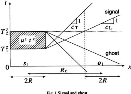
Let$S_{s}$and$S_{o}$bedisjoint spherical domainswithradiusof$R$centred at$s$and$0$,respectively.Thedistance between

$s$and$0$,

or

$|\mathit{0}-s|$,willbedenoted by$R_{c}(>2R)$

.

Also,

assume

that$S_{s}$ includesapartof$S$denoted by

S..

We

are

now

interestedin evaluatingthesingleanddoublelayerpotentials producedbydensities$t$and_$u$

on S.

$\mathrm{x}(0,t]$ and

observedat$(x,t)(x\in s_{o}, t\in(0,\infty))$

.

Eq.(13) shows that the plane

wave

expansion

for thefundamental solution includes anon-physical ghost. In

utilising thisexpansion

we

havetodevelop

an

approachwhich guarantees that the ghost doesnotpollutethe solution.

Inordertoobtain such

an

approach,

we

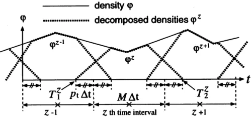
follow the developments of Erginetal. [5]to writethe density functions$u$

and$t$

as sums

of functions$u^{z}$and$t^{z}$ $(z=1, 2, \ldots)$,which have supportsinthefinite interval$(T_{1}^{z},T_{2}^{z}]$

:

$u= \sum_{z}u^{z}$, $t= \sum_{z}t^{z}$

.

Since

we

are

interested

in

aPPlying the plane

wave

expansion in

the evaluation of the the part of

integrals in

the

discretisedintegral equation in(3)which represent the effect from the past,

we

may

assume

thattheintegrals including

$u^{z}$ and$t^{z}$

are

evaluated only for_{$t>T_{2}^{z}$}

.

As

one sees

from Fig. 1the signal from$s_{s}\mathrm{x}(T_{1}^{z},T_{2}^{z}]$ reaches $S_{o}$ after

$t=T_{2}^{z}$ if

$R_{c}-2R\geq c_{L}(T_{2}^{z}-T_{1}^{z})$ (14)

holds. One also

sees

that theghost will

never

pollutethe solution if the conditionin(14)is satisfied sincetheghost

will vanishbefore the arrival of the signal.

$x$

Fig. 1Signalandghost

If the conditionin(14) _issatisfied,

one

can

evaluatepotentialfunctionsin elastodynamicsfor$(xx, t)(x\in S_{o},t>$

T22)and known densities$t^{z}$and$u^{z}$ in (S. $\mathrm{x}$ $(T_{1}^{z},T_{2}^{z}])$via

$\int_{S}$

.

$(T_{\dot{l}j}(x, y,t)*u_{j}^{z}(y, t)-\Gamma_{\dot{|}j}(x-y,t)*t_{j}^{z}(y,t))dS_{y}$

$=$ $- \frac{\partial_{t}}{8\pi^{2}}\int_{S_{k}}[k_{\dot{*}}\delta(t- (xx -s)\cdot k/c_{L})*\mathcal{O}^{z}(s, t, k)+e_{p’ k}k_{p}\delta(t-(xx -s)\cdot k/c_{T})*\mathcal{O}_{k}^{z}(s,t,k)]dS_{k}(15)$

where the functions$O^{z}$and_{$O_{k}^{z}(k=1,2,3)$},called outgoing

rays,

are

definedby

$\mathcal{O}^{z}(s,t, k)$

$=$ $\int_{S}$

.

$( \frac{C_{jlnm}n_{\mathrm{t}}k_{m}k_{n}}{\mu_{L}^{4}}\dot{u}_{j}^{z}(y,t-(s-y)\cdot k/c_{L})-\frac{k_{j}}{\rho d_{L}}t_{j}^{z}(y,t-(s-y)\cdot k/c_{L}))dS_{y}$, (16a)

(5)

$\mathcal{O}_{k}^{z}(s, t, k)$

$=$ $\int_{S}$

.

$( \frac{C_{jlnm}n_{l}e_{qmk}k_{q}k_{n}}{\rho c_{T}^{4}}\dot{u}_{j}^{z}(y,t-(s-y)\cdot k/c_{T})-\frac{e_{q\mathrm{j}k}k_{q}}{\rho c_{T}^{3}}t_{j}^{z}(y, t-(s-y)\cdot k/c_{T}))dS_{y}$

.

(16b)

Theoutgoing

rays

are

consideredtobe thetimedomain counterparts of themultipolemomentsintheFast Multipole

Method(FMM)._{Notice that the elastodynamic potential functions}

_{are now}

_expressed_in_terms_of_4components(one

from$O$ andthree from$\mathcal{O}_{k}$)of theoutgoing

rays.

The

same

property has beenobservedin elastostatics

as

well

as

in

elastodynamics in frequencydomain[2].

For$(x, t)(x\in S_{o},t>T_{2}^{z})$

one

can

_furtherrewrite₍₁₅₎_into

$\int_{S}$

.

$(T_{ij}(x, y, t)*u_{j}^{z}(y,t)-\Gamma_{ij}(x-y, t)*t_{j}^{z}(y, t))dS_{y}$

$=$ $- \frac{1}{8\pi^{2}}\int_{S_{k}}[k_{i}\delta(t-(x-\mathit{0})\cdot k/c_{L})*\mathrm{I}^{z}(\mathit{0}, t, k)+e_{pik}k_{p}\delta(t-(x-\mathit{0})\cdot k/c_{T})*\mathrm{I}_{k}^{z}(\mathit{0},t, k)]dS_{k}(17)$

where thefunctions$\mathrm{I}^{z}$ and

Ij

$(k=1,2, 3)$,called theincoming rays,

are

defined by

$\mathrm{I}^{z}\mathrm{S}\mathrm{o},\mathrm{t}k)$ $=$ $\mathcal{T}(\mathit{0}-s, t, k;c_{L})*O^{z}(s, t, k)$, (18a)

$\mathrm{I}_{k}^{z}(\mathit{0}, t, k)$ _$=$ _{$\mathcal{T}(\mathit{0}-s, t, k;c\tau)*\mathcal{O}_{k}^{z}(s,t, k)$}

.

(18b)

and

$\mathcal{T}(\mathit{0}-s,t, k;c)=\partial_{t}\delta(t-(\mathit{0}-s) \cdot k/c)$

.

Theincoming

rays

are

conceptually similartothecoefficients of the localexpansionin FMM.Also,theexpansionin

(17) andthe relations in(18)

are

_{considered to be the}_time_{domain counterparts of the local}_expansion_and _the$\mathrm{M}2\mathrm{L}$

relationintheoriginalFMM.

Finally one

sums

up thecontributionsfrom the $z\mathrm{t}\mathrm{h}$ time intervals givenby (17)to compute the

elastic potential

dueto$u$and$t$definedin_{$S_{*}\mathrm{x}(0, t]$} andobservedat

$x\in So,t>T_{2}^{z}$ by

$\int_{S_{\mathrm{s}}}(T_{ij}(x, y, t)*u_{j}(y, t)-\Gamma_{ij}(x-y,t)*t_{j}(y,t))dS_{y}=-\sum_{v=1}^{z}\frac{1}{8\pi^{2}}$

$\mathrm{x}$

$\int_{S_{k}}[k_{i}\delta(t-(x-\mathit{0})\cdot k/c_{L})*\mathrm{I}^{v}(\mathit{0}, t, k)+e_{\mu k}k_{p}\delta(t-(x-\mathit{0})\cdot k/c_{T})*\mathrm{I}_{k}^{v}(\mathit{0}, t, k)]dS_{k}$

.

(19)

3 PWTD

Algorithm for elastodynamics

In this section

we

shall describe amulti-level PWTD algorithm for elastodynamics in$3\mathrm{D}$ using

an

$\mathrm{o}\mathrm{c}\mathrm{t}$-tree structure

of theboundaryelements and the plane

wave

expansionof the potentials. We shall also discuss thecomplexityof the

algorithm.

3.1 Computation

of the

outgoing

rays

We

now

describe how

we

evaluate theoutgoing raysin(16)usingthenotation$\varphi(t)$for either of the densityfunctions

$u$

or

$t$

.

Wefirst discuss how

we

panition$\varphi$intothe

sum

of$\varphi^{z}$ which is

nonzero

only in $(T_{1}^{z},T_{2}^{z}]$

.

We

assume

that

$\varphi$is

very

smooth,

or

isband limited by$\omega_{\max}$

.

Thetime increment At isthenchosen

as

$\Delta t=\pi/\omega_{f}$ with$\omega_{f}=\chi_{1}\omega_{\max}$,

where$\chi_{1}(>1)$stands for the

over

samplingratio. As Erginetal.suggest_[5],

we

interpolate$\varphi$using

an

approximately

timeandbandlimitedbase function$\psi(t)$

as

$\varphi(t)\simeq\sum_{\alpha}\varphi(\alpha\Delta t)\psi(t-\alpha\Delta t)$ (20)

and

group

consecutive$M$termstogether todefine

$\varphi^{z}(t)=\sum_{\alpha=(z-1)M+1}^{zM}\varphi(\alpha\Delta t)\psi(t-\alpha\Delta t)$

.

(21)

(6)

We thussplit$\varphi$into

asum

ofapproximately timeandbandlimited functions

$\varphi^{z}$with thehelpof$M$samples of$\varphi$

.

For

the present

purpose,

Erginetal.[5]suggestto

use

thefollowingfunction for$\psi$

:

$\psi(t)=\frac{\omega_{0}}{\omega_{f}}\frac{\sin(\omega_{0}t)}{aJ_{0}t}\frac{\sin(\Omega p_{t}\Delta t\sqrt{(t/p_{t}\Delta t)^{2}-1})}{\sinh(\Omega p_{t}\Delta t)\sqrt{(t/p_{t}\Delta t)^{2}-1}}$

(22)

where$\omega_{0}=\omega_{\max}(\chi_{1}+1)/2$,$\Omega=\omega_{\max}(\chi_{1}-1)/2$,and$p_{t}>0$is

an

integer.In(22)

we

interpret$\sqrt{(t/pt\Delta t)^{2}-1}=$

$i\sqrt{1-(t}/p_{t}\Delta t)^{2}$ when $t<p_{t}\Delta t$

.

Itis

seen

that $\psi$isband limited by $\omega f$ and almost vanishes for$|t|>p\iota^{\Delta t}[5]$

.

Hence,$\varphi^{z}$is certainlyband limited andapproximately timelimited. Since

one

has

$T_{1}^{z}=((z-1)M+1-p_{t})\Delta t$, $T_{2}^{z}=(zM+p_{t})\Delta t$ (23)

from(21),

one sees

that thecondition

in

(14)

is

satisfied if

one

sets$M$

so

that

$M \leq\frac{R_{\mathrm{c}}-2R}{c_{L}\Delta t}-2p_{l}+1$ (24)

holds. The parameter$p_{t}$ isselectedappropriatelyconsidering the

accuracy

and efficiencyoftheanalysis. One

may

generally

say

that alarge$p_{t}$ will be desirable fiom thepointofviewof the

accuracy

of(20),while taking$Pt$toolarge

willmake$M$in₍₂₄₎small

or

even

negative,thus making the analysis inefficient.

With$\varphi^{z}$thusconstructed,

one

may

use

anumerical quadrature

on

boundary elements and thedefinition in(16)to

compute theoutgoing

rays

producedby densities

on S..

Thetimederivative for$u^{z}$ includedin(16)

may

easily be

obtainedwith thehelp of FFT.

In thesequel,

we

shall call the time interval$((z-1)M\Delta t, zM\Delta t](z=1,2, \ldots)$the zthtimeinterval. Notice that

thistime interval is includedin$(T_{1}^{z},T_{2}^{z}]$

as one can see

in Fig. 2.

$\mathrm{d}\mathrm{e}\mathrm{n}\mathrm{s}\dot{|}\mathrm{t}y\varphi$

Fig. 2Decomposition of adensity$\varphi$to$\varphi^{z}$

3.2 Discretisation of

integrals

on

the

unit

sphere

In the numerical analysis the integral

on

the unit sphere $s_{k}$ in (17) hasto be evaluated with acertain numerical

integration. Itisobviously

necessary

toselect

an

appropriateset of$k\mathrm{s}$

as

theintegration points. Areasonablechoice

is obtained

as one

considers the

process

ofcomputingtheoutgoingandincoming

rays.

We rememberthat the densities$u^{z}(t)$ and$t^{z}(t)$

are

band-limitedto$\omega f$,

so

thatthe wavenumber of the densities

isestimatedtobe$\omega_{f}/c$atthe largest, where$c$isthe velocity of the relevant

wave.

Therefore theoutgoing

rays

from

sources

distributed in the

source

sphere$S_{s}$,which has radius of$R$,will berepresentedbysphericalharmonicsof the

orderof

$K= \frac{2R\omega_{f}\chi_{2}’}{c_{T}}$

.

(25)

$(\mathrm{c}\mathrm{f}c\iota >c_{T})$

.

Theintegral

on

theRHS of(19)

is

now

approximated

as

$\int_{S}$

.

$(T_{\dot{|}\mathrm{j}}(x,y,t)*u_{j}^{z}(y,t)-\Gamma_{\dot{|}j}(x-y,t)*t_{\mathrm{j}}^{z}(y,t))dS_{y}$

(7)

$\simeq$ $- \frac{1}{8\pi^{2}}\sum_{p=0}^{K}\sum_{q=-K}^{K}w_{pq}[(k_{pq})_{i}\delta(t-(x-\mathit{0})\cdot k_{pq}/c_{L})*\mathcal{T}(\mathit{0}-s, t, k_{pq};c_{L})*\mathcal{O}^{z}(s, t, k_{pq})$

$+e_{jik}(k_{pq})_{j}\delta(t-(x-0)\cdot k_{pq}/c_{T})*\mathcal{T}(\mathit{0}-s, t, k_{pq};c_{T})*\mathcal{O}_{k}^{z}(s, t, k_{pq})]$

$=$ $- \frac{1}{8\pi^{2}}\sum_{p=0}^{K}\sum_{q=-K}^{K}w_{pq}[(k_{pq})_{i}\delta(t-(x-\mathit{0})\cdot k_{pq}/c_{L})*\mathrm{I}^{z}(\mathit{0}, t, k_{pq})$

$+ejik(k_{pq})_{j}\delta(t-(x-0)\cdot k_{pq}/c_{T})*\mathrm{I}_{k}^{z}(s, t, k_{pq})]$

(26)

(27)

where$k_{pq}$,$w_{pq}$,$\theta_{p}$and$\phi_{q}$$(p=0, \ldots, K, q=-K, \ldots, K)$

are

defined by

$k_{pq}$ $=$ $\sin\theta_{p}\cos\phi_{q}i_{1}+\sin\theta_{p}\sin\phi_{q}:_{2}+\cos\theta_{p}:_{3}$, (28a)

$w_{pq}$ $=$ $\frac{4\pi\sin^{2}\theta_{p}}{(2K+1)[(K+1)P_{K}(\cos\theta_{p})]^{2}}$, (28b)

$\theta_{p}$ $=$ $(p+1)$throotofequation$P_{K+1}(\cos\theta)=0$, (28c)

$\phi_{q}$ $=$ $\frac{2\pi q}{2K+1}$ $(28\mathrm{d})$

intermsof the orthonormal base vectors :for thecartesiancoordinateaxis.

3.3 Description of the algorithm

To solve the BIEgiven by(3),

we

havetoevaluate elastic potentials with known densities. In fast algorithms of the

multi-level FMM tyPeto evaluate thesepotentials atapoint $x$,

we

split the boundary intotwo parts: i.e. the part

$s_{f}^{(l)}(xx)$whichisfarfrom$xx$and$S_{n}^{(\mathrm{t})}(x)=S$$\backslash S_{f}^{(l)}(x)$ whichisclose to$x$

.

Thecontributionstothepotentialsfrom

$S_{f}^{(\mathrm{t})}(x)$iscomputed with the help of the plane

wave

expansion,while the evaluation of the contributions from$S_{n}^{(l)}(x)$

ispassedto$l+1\mathrm{t}\mathrm{h}$level. At the deepest level(largest$l$),

we

compute the contributions from$S_{n}^{(l)}(x)$directlyusingthe

conventional methods.

Todescribe this algorithm

more

precisely,

we

havetodefine what

we mean

by the words ‘far’ and ‘level’. We first

discretise the boundary integral equation(3)_{using boundary elements having}$N_{s}$ spatial degrees of freedom and$N_{t}$

timeintervals of the length At. Fordefiniteness,

we

assume

theboundary elementstobepiecewiseconstantandthe

timebasefunctionstobepiecewiselinear,although theseassumptions

are

notessential.

Wenextconstructthe$\mathrm{o}\mathrm{c}\mathrm{t}$-treestructureof boundary elementsin the following

manner.

Wefirst take acube which

includesthe domain$D$

.

Thiscube is called the cell of the level0. This cube is subdivided into 8equalsub-cubes,

of which thosecontainingboundary elements

are

called cells of the level 1. Werepeatthissubdivision until the cell

contains less than afixed number(denotedby$N_{cell}$)ofboundary elements. Acell without childreniscalledaleaf,

andthe level number of the deepest cell is denoted by$l_{\max}$

.

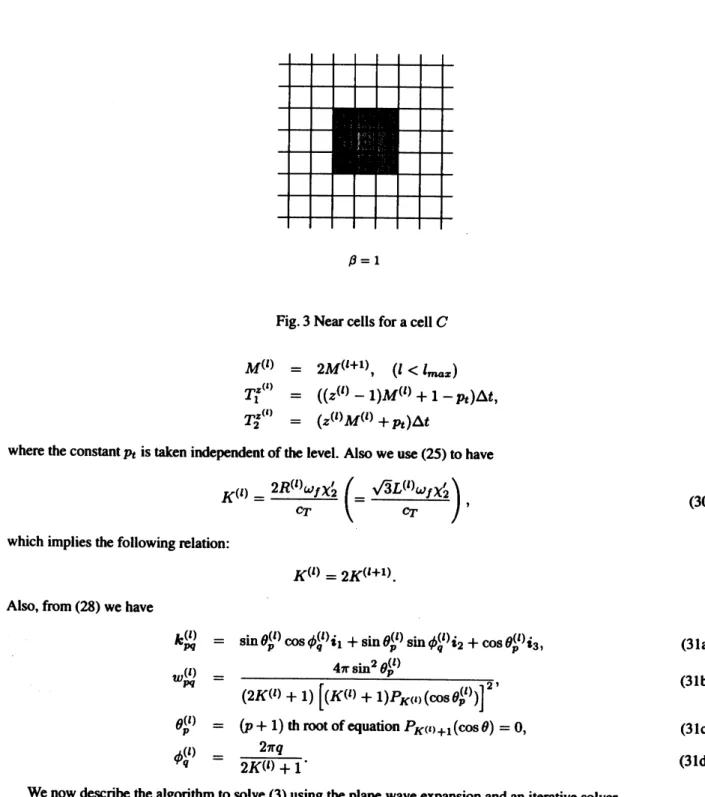
We

say

twocells$C$and$C’$of the level$l$tobe close if

$|C_{\dot{l}}-C’.\cdot|<(\beta+1)L^{(l)}$ $i=1,2$, 3 (29)

holds,where$c_{\dot{l}}$ and$C_{\dot{1}}’$

are

the coordinatesof the centroids of$C$and $C’$,$\beta$isanatural number and$L^{(l)}$ istheedge

length of the level$l$cell. With thisdefinition, theset$S_{n}^{(l)}(x)$ isdefinedto be theunionof level$l$cells $C’$which is

closeto$C$if$x\in C$

.

The cells$C’$of the level$l$which

are

notclose to$C$

are

saidtobefar from$C$

.

In Fig.3

we

have

indicated cells closetothe cell$C$when$\beta$isequalto 1. In therestof this

paper

we

shall

assume

that$\beta=1$

.

In the evaluation of elastic potentialsatapoint$x$ in alevel$l$cell$C$,

we

shall

use

theplane

wave

expansionwhen

we

computetheeffects from boundary elements includedinalevel$l$cell $C’$whichisfar from$C$

.

Thecontributions

fromfar cells

are

evaluatedin the form of theincoming raysassociated with$C$

.

To compute contributions from cells far from$C$,

we

havetodetermine,foreach level 1, numbers$R^{(\mathrm{t})}$,$R_{\mathrm{c}}^{(l)}$,$T_{1}^{z^{(1)}}$,

$T_{2}^{z^{(1)}}$and$M^{(l)}$ whichsatisfy₍₁₄₎and_(24),where the superposed (/) indicates that the associatedquantityisfor level

$l$cells. Itisconsidered naturalto set

$R^{(l)}= \frac{\sqrt{3}L^{(l)}}{2}$, _{$R_{c}^{(l)}=2L^{(l)}$},

except in (14), _{whose LHS}

_can

_{be put equal to} $\beta L^{(l)}(=L^{(l)})$, since it is sufficient to set the LHSof(14)

as

the

minimumdistance between$S_{o}$and$S_{s}$

.

Accordingly,

one

puts$M^{(l)}$,$T_{1}^{z^{(l)}}$ and$T_{2}^{z^{(\mathrm{t})}}$

tobe

$M^{(l_{\max})}$ _$=$ $\frac{L^{(\mathrm{t}_{\max})}}{c_{L}\Delta t}-2p_{t}+1$,

(8)

$\beta=1$

Fig. 3Nearcells for acell$C$

$M^{(\mathrm{t})}$ $=$ $2M^{(l+1)}$, $(l<l_{\max})$ $T_{1}^{z^{(\downarrow)}}$ $=$ $((z^{(l)}-1)M^{(l)}+1-p_{t})\Delta t$, $T_{2}^{z^{(I)}}$ $=$ $(z^{(l)}M^{(l)}+p_{\mathrm{C}})\Delta t$

where the constant$pt$ istakenindependent of the level. Also

we

use

(25)tohave

$K^{(l)}= \frac{2R^{(l)}\omega_{f}\chi_{2}’}{c_{T}}(=\frac{\sqrt{3}L^{(l)}\omega_{f}\chi_{2}’}{c_{T}})$ , (30)

whichimpliesthefollowingrelation:

$K^{(l)}=2K^{(l+1)}$

.

Also,_from(28)

we

have

$k_{\mathrm{p}q}^{(l)}$ $=$ $\sin\theta_{p}^{(\mathrm{t})}\omega \mathrm{s}\phi^{(l)}q:1+\sin\theta_{\mathrm{P}}^{(l)}\sin\phi_{q}^{(l)}:_{2}+\cos\theta_{p}^{(l)}:_{3}$, (31a)

$w_{\mathrm{N}}^{(l)}$ $=$

$\frac{4\pi\sin^{2}\theta_{p}^{(l)}}{(2K^{(l)}+1)[(K^{(l)}+1)P_{K\mathrm{t}}\mathrm{t})(\cos\theta_{p}^{(l)})]^{2}}$, (31b)

$\theta_{p}^{(l)}$ _$=$ $(p+1)$throotofequation

$P_{K^{(2)}}\dagger 1(\cos\theta)=0$, (31c)

$\phi_{q}^{(l)}$ $=$ $\frac{2\pi q}{2K^{(l)}+1}$

.

$(31\mathrm{d})$

We

now

describethe algorithmtosolve(3)usingthe plane

wave

expansionand

an

iterative

solver.

1. Initial

guess

Let thecurrenttime be$t_{\alpha}=\alpha\Delta t$ $(\alpha=1, 2, \ldots, N_{t})$ andall theboundary displacements_and_{tractions in}_the

past,i.e.$u(\cdot,t_{\alpha’})$ and$t(\cdot,t_{\alpha’})$for$t_{\alpha’}(\alpha’=1, \ldots,\alpha-1)$,

are

known.

We then provide initial

guesses

tothe unknown parts of$u(\cdot,t_{\alpha})$ and$t(\cdot$,$t_{\alpha})$arbitrarily. Givingthe values for

the

same

quantitiesat$t_{\alpha-1}$ wouldbe areasonable choice.

2. Evaluationof potentials dueto

sources on

$S\mathrm{x}(0, t_{\alpha}]$

As the densityfunctions

on

$S\mathrm{x}(0,t_{\alpha}]$

are

given,the potentialsin(3)for each collocationpoint

$x$dueto

sources

on

$S\mathrm{x}(0,t_{\alpha}]$

are

dividedintocontributions from the

near

part$S_{||}^{(l)}(x)\mathrm{x}(0,t_{\alpha}]$ andfarpart$S_{f}^{(l)}(x)\mathrm{x}(0,t_{\alpha}]$

.

$2\mathrm{a}$

.

Conhibutions

from the

near

part$S_{n}^{(\mathrm{t})}(x)\mathrm{x}(0,t_{\alpha}]$

For each cell(denotedby$C$) of the level$l(l\geq 2)$_,

use

_{the conventional direct}_integration_{to compute}

contri-butions to the elastic potentialsatthe collocationpoints $(x, t_{\alpha})(x\in C)$from densities $u(\cdot, t_{\alpha’})$ and$\mathrm{t}$($-$,ta)

$(\alpha’=1, \ldots, \alpha)$distributedin

a

neighbouring cell$C’$of the level$l$(including_$C$

itself)if either$C$

or

$C’$isaleaf

(9)

$2\mathrm{b}$

.

Contributionsfrom the far

part$S_{f}^{(\mathrm{t})}(x)\mathrm{x}(0, t_{\alpha}]$

Let$l$be the level of the leaf containing

$x$

.

We notethefollowing: for alevel $l$cell,the time$t_{\alpha}$belongstothe

$z_{\alpha}^{(l)}\mathrm{t}\mathrm{h}$

timeinterval, where $z_{\alpha}^{(l)}=\lfloor\alpha/M^{(l)}\rfloor$ and $\lfloor\cdot\rfloor$ stands for the ‘floor’operation. At$t_{\alpha}$ theoutgoing

rays

$\mathrm{o}^{z^{(l)}}$

(intherestof this

paper we

shall

use

acollectivenotation$0^{z^{(l)}}$

for ($\mathcal{O}^{z^{(\mathrm{t})}}$

,$\mathcal{O}_{i}^{z^{(l)}}$)) and theincoming

rays

$\mathrm{I}^{z^{(1)}}$

correspondingto$z^{(l)}=1,2$,$\ldots$,

$z_{\alpha}^{(\mathrm{t})}-1$

are

all known(seetheprocedure in$4\mathrm{b}$below). Theincoming rays

$\mathrm{I}^{z^{(l)}}$

determine the layer potentials duetodensities$u^{z^{(l)}}$

and$t^{z^{(l)}}$ distributedin

$S_{f}^{(l)}(x)\mathrm{x}(T_{1}^{z^{(l)}}, T_{2}^{z^{(l)}}]$via(27),

which

we

have had already computed instep$4\mathrm{b}$

.

Namely, atthecollocationpoint _{$(x, t_{\alpha})$} thelayer potentials

due to densities$\sum_{z^{(l)}=1}^{z_{\alpha}^{(l)}-1}u^{z^{(\mathrm{t})}}$ and$\sum_{z^{(l)}=1}^{z_{\alpha}^{(l)}-1}t^{z^{(l)}}$

on

$S_{*}\mathrm{x}(0, T_{2}^{z_{\alpha}^{(l)}-1}]$ have been computed and stored. Onejust

recalls the values thus stored. We note that thepotentialsdue todensities distributed

on

$S_{f}^{(\mathrm{t})}(x)\mathrm{x}(T_{2}^{z_{\alpha}^{(l)}-1},t_{\alpha}]$

will not reach collocationpoints$(x,t_{\alpha})$ before$t=T_{2}^{z_{\alpha}^{(l)}}$,

and do nothave to be takeninto consideration. We

have thus evaluated potentials due to densitiesin$S_{f}^{(l)}(x)\mathrm{x}(0, t_{\alpha}]$

.

3. Determination of thecurrentunknowns

We update the unknownsat$t=t_{\alpha}$following the procedures oftheiterative solver used and returnto step 1

if the discretised version of the BIE in(3)isnotsatisfied to within

an

allowable

error.

Otherwise the assumed

values for the unknownsat$t=t_{\alpha}$

are

adopted

as

thesolution at ta. If$\alpha<N_{t}$

we

go

tostep4. Otherwise

we

terminatetheanalysis.

4. Computation ofoutgoing raysandincoming rays

Compute theoutgoingandincoming

rays

for$z_{\alpha}^{(l)}$

in the following

manner:

$4\mathrm{a}$

.

Computataionof theoutgoing

rays

(upward)

Startingfrom leaves

up

tolevel 2cells

we

computetheoutgoing

rays

$\mathit{0}^{z_{\alpha}^{(l)}}$

atthecentroid of the cellforthe

$z_{\alpha}^{(l)}\mathrm{t}\mathrm{h}$

time intervalif andonly ifthe currenttime stepnumber$\alpha$ is amultiple of$M^{(l)}$. To compute

$\mathit{0}^{z_{\alpha}^{(l)}}$

we

use

thedefinition in(16)if$C$is aleaf. For non-leaf cells

we

add theoutgoingraysof the child cells$\mathit{0}^{z_{\alpha}^{(\mathrm{t}+1)}-1}$

and $\mathit{0}^{z_{\alpha}^{(1+1)}}$

after shifting thecentresof the expansion from those of the children $(s’)$to that of$C(s)$

.

_Since

uppercellsrequire

more

directions(k) than the lower

ones

because of(30),

_we

have toincrease the number

of directions

as we go up

thetree structureof cells. Tocopewiththisrequirement

we use an

operation called

‘interpolation’.See[5]_{for the detail.}

$4\mathrm{b}$

.

Computation oftheincoming

rays

(downward)

Starting from level 2cells

we

computetheincoming raysfor thecurrent$(z_{\alpha}^{(\iota)}\mathrm{t}\mathrm{h})$time interval

atthecentroids of

level$l$cells if and only if the

currenttimestepnumber$\alpha$is amultiple of$M^{(l)}$,

as

instep$4\mathrm{a}$

.

Inthis

process we

define theincoming raysassociated with alevel$l$cell$C$tobe the

sum

of theincoming raysfrom all the level$l$

cells(denotedcollectively by$C’$₎which

are

_notcloseto$C$

.

Such$C’\mathrm{s}$consistof level$l$cellswhich

are

notclose

to$C$but whoseparents

are

closetothe parent of$C$(interaction list)andthose whose parents

are

notclosetothe

parentof$C$

.

The contributionsto$\mathrm{I}^{z_{\alpha}^{(l)}}$

from the former(cells_{in the}_interactionlist of$C$)

are

evaluatedvia(18),

butinthefrequencydomainusingasmoothed$\mathcal{T}$(See [5]). On the otherhand,thecontributions ffom the latter

$C’\mathrm{s}$

are

obtained

as

one

shifts the incoming raysof the parent of$C(\mathrm{I}^{z_{\alpha}^{(l-1)}})$ from the centroid of the parent

$(\mathit{0}’)$tothat of$C(0)$. Notice that the number of directions$k$ required for$C$ is lessthanthatpossessed by the

parent. Therefore

one

has to ‘anterpolate’ theincoming raysin the downward path of the algorithm[5]. When

$C$isaleaf,

one

uses

theincoming raysfor$C$thusobtained$(\mathrm{I}^{z_{\alpha}^{(l)}})$

and(27)tocomputethe elastic potentials for

$t>T_{2}^{z_{\alpha}^{(\mathrm{t})}}$

dueto$u$and$t$inthepastdistributedin far cells. Thecomputation iscarriedoutinthe ‘castforward’

manner

withrespect to time,and stored. The results will be recalledin step$2\mathrm{b}$later.

5. Update

Update$\alpha$by$\alpha+1$and

go

to step 1.

.4

Complexity

of

the algorithm

$t\mathrm{e}$consideraseriesof problemswithincreasingdomainsizesolved with the

same

accuracy

(i.e.the number of

nodes

$\underline{\sim}\mathrm{r}$

wave

lengthremainsconstant). Ergin etal. [5] estimated that the complexity of their PWTD algorithm for the

ave

equationin$3\mathrm{D}$appliedtotheseriesof problems of thistyPeis_{$O(N_{s}\log^{2}N_{s}N_{t})$}

.

Usingthe

same

argument

as

1Erginetal.,

_one

_{shows that the complexity of the}_part_{of the}_present_{algorithm using the plane}

_wave

_expansion_is

(10)

identical with that ofErginet al.Onealsoshows that the directcomputationpart of theelastodynamic algorithmscales

as

$O(N_{s}N_{t})$inspiteof thetime integrationincludedinthepotential representationof the solution. Thisisbecause the

elastodynamic fundamental solution in $3\mathrm{D}$ vanishes after the time required for$\mathrm{S}$

waves

generatedatthe collocation

point$x$to

sweep

outthe part of the boundary where the contributiontothepotentialsat$x$isevaluated directly. One

therefore concludes that the overallcomplexityof theproposed approach is$O(N_{s}\log^{2}N_{s}N_{t})$ if

one

followsclosely

the approachproposedbyErginetal.

Erginetal., however,

assumes

that they

use

fast method of evaluating the Legendre transform[6]in the

interpola-tionandanterpolationtoestablish theircomplexity estimate. Since

our

implementation

uses

thestandard(sometimes

called.semi-fast algori thm[6]for this

purpose,

however,

our

algorithmcannotbe faster than$O(N_{s}^{3/2}N_{t})$

.

In

prob-lemsof thesize considered in this

paper,

it

may

notbeobvious if the

use

of ’fast’ methods for the Legendre transform

actuallyimprovestheperformance ofthealgorithm

or

not.

4Numerical analysis

4.1 Details

of the

present implementation

Inthe following examples

we use

GMRES withoutpreconditioning

as

the iterativesolver to obtain the solution of

discretisedversionof(3)in both fast and conventional BIEM. As the initial

guess,

we

use zero

for the first time step,

and the solutions at theprevioustimestep for the rest of analysis

Ashas beenseen,

our

implementationrequiresthe following parameters: $N_{ce}\iota\iota$:maximumnumber of boundary

elements in aleaf cell(see3.3),$n$:parameters relatedtothe interpolation functions with respecttotime(see(22)),$\chi 1$

:

over

samplingrate,At: time increment whichisrelatedtothemaximum frequencyof the fieldquantities$\omega_{\max}$ by

$\omega_{\max}=\pi/(\chi_{1}\Delta t)$and$\chi_{2}’$:aparameter relatedtothe number of directions$k$(see(25)).The following choices of the

parameters

are

used in theexamplesgivenbelow: $\chi_{1}=3.0$,$\chi_{2}’=0.2$and$p_{t}=3$

.

This choice for$\chi_{1}$

means

that

one

uses

6timenodes

per

theshortest of theexpected periods.Also,

we

have used

an

appropriate non-dimensionalisation

to set$cL=1$,$c\tau$ $=1/\sqrt{2}$and$\rho=1$

.

This

means

that the Poisson’sration is equalto

0.

In thecomputation

we

haveused Fujitsu$\mathrm{V}\mathrm{P}\mathrm{P}800/63$ with$7\mathrm{G}\mathrm{B}$of the mainmemory.Thecodeisnotparallelised.

4.2 Numerical example

(32)

Weconsider

as

thedomain$D$ parallelepiped having the lineconnecting(0,0,0)and$(X,\mathrm{Y}, Z)$

as

the

space

diagonal.

Inthe initial boundary value problemconsidered,theinitialdisplacement and velocity

are

assumed to vanish. As the

boundary condition

we

prescribethetraction computedfiom thefollowingfield:

$u(x,t)=d[1$ -Cos$\frac{2\pi}{\Lambda}(t-\frac{d\cdot x}{c_{L}})]$ ,

where$d$isaunitvectorand thefunctionCos is definedby

$\mathrm{C}\mathrm{o}\mathrm{s}x=\{$

$\infty \mathrm{s}x$ $0\leq x\leq 2\pi$

1 $x<0$, $x>2\pi$ (33)

Thefunction$u$obviously represents aplane$\mathrm{P}$

wave

propagatinginto the direction$d$

.

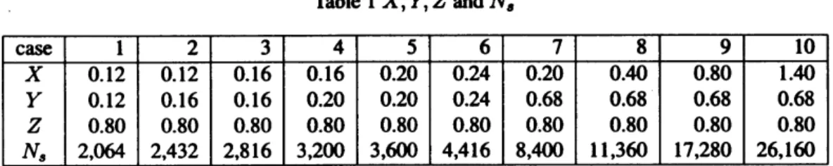
The solutiontothe problem

underconsiderationisobviously$u$itself. Weset$d=(0, 0, 1)$,$\mathrm{A}=0.5$,$Z=0.80$and$N_{t}=2\alpha$].For the parameters

$X$and$\mathrm{Y}$

we

consider the 10

cases

listed in Table1. This table also shows$N_{s}$

.

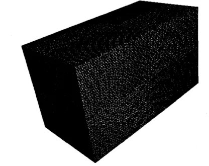
See Fig.4(thisfigure shows the

case

10 inTable1)for

an

example of the boundarydiscretisation. Other parameters

are

set

as

$\Delta t=0.\mathrm{O}1$and_{$N_{ceu}=150$}

.

Thedepth of the$\mathrm{o}\mathrm{c}\mathrm{t}$-tree_{$l_{\max}$}is equal to2in

case

2,3in

cases

2-9, and4in

case

10.We note that the choice$\chi_{2}’=0.2$

yields that the number$K^{(2)}$ tobe24 in

cases

1-9and

56

in

case

10.Thenumberof directionsinlevel 2cellsisthen

given by $(K^{(2)}+1)(2K^{(2)}+1)$

.

Table 1 $X,\mathrm{Y}$,$Z$and$N_{t}$

(11)

Fig. 4Boundary element discretisation used incase10(78,480 DOF)

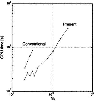
Fig.5showsthe CPUtime(sec)

vs

the number of unknowns $N_{s}$

.

Thisfigure shows that the present method is

capableofcarryingoutelastodynamic analysisin timedomain

more

efficientlythan the conventional methodinall the

examples considered. The fluctuation of theCPUtimeforsmall$N_{s}$

seems

tobedue to the condition of the computer,

whichisshared bymanyusers.

Because of therestriction of the memoryit

was

not possibleto solve

cases

5-10 with the conventional BIEM.

IfCPUtime isnotimportant, however,

one

may

use

the conventional method in larger problems by not storingall

the integration results, but by recalculating them when needed. In thisway

we

could solve all the

cases

with the

conventional approachusing adesktopcomputer(Alpha21264 (600[MHz]), $2[\mathrm{G}\mathrm{B}]$ofmemory),and could

compare

the results of the proposed and conventional approaches in all

cases.

It

was

found that the maximum

error

of the

boundary displacements(relativetothemaximum boundary displacement$(=2)$)

was

about3% in both proposed and

conventional methods.

Wefinally remark that the following url includes animations of other examples solved with the proposed method.

http:$//\mathrm{g}\mathrm{e}\mathrm{e}\mathrm{h}\mathrm{o}\mathrm{s}\mathrm{t}$.gee

.

$\mathrm{k}\mathrm{y}\mathrm{o}\mathrm{t}\mathrm{o}-\mathrm{u}.\mathrm{a}\mathrm{c}$

.

$\mathrm{i}\mathrm{p}/\sim \mathrm{t}\mathrm{t}\mathrm{a}\mathrm{k}\mathrm{a}/\mathrm{e}\mathrm{a}\mathrm{b}\mathrm{e}$ .html

5Conclusion

Inthis

paper we

could successfully extend the PWTD algorithm proposed for the

wave

equationbyErginetal. [5]to

elastodynamicsin$3\mathrm{D}$

.

We could also show the effectiveness of the proposedapproach insimpletestproblems of the

spatialsize of$O(10^{4})$

.

Since the method isstill inits incipientstage of developments

we

still needtorefine the code

so

thatit

can

be

appliedtolarger problems found in engineeringapplications. However, thefundamentals of the approach

are now

established and the numerical results

seem

tobepromising.

References

[1] _{Kobayashi S}_et_al.._{Wave Analysis and Boundary Element Methods. Kyoto}_UniversityPress;2000(in Japanese).

[2] Nishimura N. Fastmultipoleacceleratedboundary integralequationmethods.acceptedforpublicationin Applied

MechanicsReviews2002.

[3] TakahashiT,NishimuraN,Kobayashi S. Fast boundary integralequationmethod for elastodynamicproblemsin

2Din timedomain. Trans JSME$2\propto 11j\mathrm{A}67- 661:14\{\mathrm{D}-16$(in Japanese).

(12)

$\overline{\underline{\infty}}$

$.\vee\underline{\Phi\in}$

$\mathrm{o}\mathrm{L}\supset$

Fig. 5Comparisonof computationaltime

[4] Lu M,WangJ, ErginAA,Michielssen E. Fastevaluation of

tw0-dimensional transient

wave

fields. J Comput

Phys2000;

158:161-85.

[5] ErginAA,ShankerB,Michielssen E. Fast analysis oftransient acoustic

wave

scatteringfrom rigid bodiesusing

the multilevel plane

wave

time domain algorithm. J Acoust Soc Am$2\propto \mathrm{K}1;107:1$168-78.

[6] ChienRJ,Alpert BK. Afast spherical filter with uniform resolution. JComputPhys 1997;136:580-4