Strong instability of standing waves
for nonlinear Schr¨
odinger equations
with double power nonlinearity
Masahito Ohta and Takahiro Yamaguchi
(Received July 3, 2014; Revised November 10, 2014)
Abstract. We prove strong instability (instability by blowup) of standing waves for some nonlinear Schr¨odinger equations with double power nonlinearity.
AMS 2010 Mathematics Subject Classification. 35Q55, 35B35.
Key words and phrases. Nonlinear Schr¨odinger equation, standing wave, blowup, instability.
§1. Introduction
In this paper, we study instability of standing wave solutions eiωtϕω(x) for
nonlinear Schr¨odinger equations with double power nonlinearity:
i∂tu =−∆u − a|u|p−1u− b|u|q−1u, (t, x)∈ R × RN,
(1.1)
where a and b are positive constants, 1 < p < q < 2∗− 1, 2∗= 2N/(N − 2) if
N ≥ 3, and 2∗=∞ if N = 1, 2.
Moreover, we assume that ω > 0 and ϕω ∈ H1(RN) is a ground state of −∆ϕ + ωϕ − a|ϕ|p−1ϕ− b|ϕ|q−1ϕ = 0, x∈ RN.
(1.2)
For the definition of ground state, see (1.5) below. It is well known that there exists a ground state ϕω of (1.2) (see, e.g., [2, 15]).
The Cauchy problem for (1.1) is locally well-posed in the energy space
H1(RN) (see, e.g., [3, 7, 8]). That is, for any u0 ∈ H1(RN) there exist
T∗ = T∗(u0) ∈ (0, ∞] and a unique solution u ∈ C([0, T∗), H1(RN)) of (1.1)
with u(0) = u0 such that either T∗ = ∞ (global existence) or T∗ < ∞ and
lim
t→T∗∥∇u(t)∥L2 =∞ (finite time blowup).
Furthermore, the solution u(t) satisfies
E(u(t)) = E(u0), ∥u(t)∥2L2 =∥u0∥2L2 (1.3)
for all t∈ [0, T∗), where the energy E is defined by
E(v) =1 2∥∇v∥ 2 L2− a p + 1∥v∥ p+1 Lp+1− b q + 1∥v∥ q+1 Lq+1.
Here we give the definitions of stability and instability of standing waves. Definition 1. We say that the standing wave solution eiωtϕω of (1.1) is stable
if for any ε > 0 there exists δ > 0 such that if ∥u0 − ϕω∥H1 < δ, then the solution u(t) of (1.1) with u(0) = u0 exists globally and satisfies
sup t≥0 inf θ∈R,y∈RN∥u(t) − e iθϕ ω(· + y)∥H1 < ε. Otherwise, eiωtϕ ω is said to be unstable.
Definition 2. We say that eiωtϕω is strongly unstable if for any ε > 0 there
exists u0 ∈ H1(RN) such that ∥u0− ϕω∥H1 < ε and the solution u(t) of (1.1) with u(0) = u0 blows up in finite time.
Before we consider the double power case, we recall some well-known results for the single power case:
i∂tu =−∆u − |u|p−1u, (t, x)∈ R × RN.
(1.4)
When 1 < p < 1 + 4/N , the standing wave solution eiωtϕω of (1.4) is stable
for all ω > 0 (see [4]). While, if 1 + 4/N ≤ p < 2∗− 1, then eiωtϕ
ω is strongly
unstable for all ω > 0 (see [1] and also [3]).
Next, we consider the double power case (1.1) with a > 0 and b > 0. From Berestycki and Cazenave [1], we see that if 1 + 4/N ≤ p < q < 2∗− 1, then the standing wave solution eiωtϕω of (1.1) is strongly unstable for all ω > 0
(see [14] for the case p = 1 + 4/N < q).
On the other hand, when 1 < p < 1 + 4/N < q < 2∗ − 1, the standing wave solution eiωtϕω of (1.1) is unstable for sufficiently large ω (see [13]),
while eiωtϕω is stable for sufficiently small ω (see [5] and also [12, 11] for more
results in one dimensional case). However, it was not known whether eiωtϕω
is strongly unstable or not for the case where 1 < p < 1 + 4/N < q < 2∗− 1 and ω is sufficiently large.
Now we state our main result in this paper.
Theorem 1. Let a > 0, b > 0, 1 < p < 1+4/N < q < 2∗−1, and let ϕω∈ Gω. Then there exists ω1 > 0 such that the standing wave solution eiωtϕω of (1.1) is strongly unstable for all ω∈ (ω1,∞).
For ω > 0, we define functionals Sω and Kω on H1(RN) by Sω(v) = 1 2∥∇v∥ 2 L2 + ω 2∥v∥ 2 L2 − a p + 1∥v∥ p+1 Lp+1− b q + 1∥v∥ q+1 Lq+1, Kω(v) =∥∇v∥2L2 + ω∥v∥2L2− a∥v∥p+1Lp+1− b∥v∥ q+1 Lq+1.
Note that (1.2) is equivalent to Sω′(ϕ) = 0, and
Kω(v) = ∂λSω(λv) λ=1=⟨Sω′(v), v⟩
is the so-called Nehari functional. We denote the set of nontrivial solutions of (1.2) by
Aω={v ∈ H1(RN) : S′ω(v) = 0, v̸= 0},
and define the set of ground states of (1.2) by
Gω={ϕ ∈ Aω: Sω(ϕ)≤ Sω(v) for all v∈ Aω}.
(1.5)
Moreover, consider the minimization problem:
d(ω) = inf{Sω(v) : v∈ H1(RN), Kω(v) = 0, v̸= 0}.
(1.6)
Then, it is well known thatGω is characterized as follows. Gω ={ϕ ∈ H1(RN) : Sω(ϕ) = d(ω), Kω(ϕ) = 0}.
(1.7)
The proof of finite time blowup for (1.1) relies on the virial identity (1.8). If u0 ∈ Σ := {v ∈ H1(RN) : |x|v ∈ L2(RN)}, then the solution u(t) of (1.1)
with u(0) = u0 belongs to C([0, T∗), Σ), and satisfies
d2
dt2∥xu(t)∥ 2
L2 = 8P (u(t)) (1.8)
for all t∈ [0, T∗), where
P (v) =∥∇v∥2L2− aα p + 1∥v∥ p+1 Lp+1− bβ q + 1∥v∥ q+1 Lq+1 with α = N 2(p− 1), β = N 2 (q− 1) (see, e.g., [3]).
Note that for the scaling vλ(x) = λN/2v(λx) for λ > 0, we have
∥∇vλ∥2 L2 = λ2∥∇v∥2L2, ∥vλ∥ p+1 Lp+1= λ α∥v∥p+1 Lp+1, ∥v λ∥q+1 Lq+1 = λ β∥v∥q+1 Lq+1, ∥vλ∥2 L2 =∥v∥2L2, P (v) = ∂λE(vλ) λ=1.
The method of Berestycki and Cazenave [1] is based on the fact that d(ω) =
Sω(ϕω) can be characterized as
d(ω) = inf{Sω(v) : v∈ H1(RN), P (v) = 0, v̸= 0}
(1.9)
for the case 1 + 4/N ≤ p < q < 2∗− 1. Using this fact, it is proved in [1] that if u0 ∈ Σ ∩ BωBC then the solution u(t) of (1.1) with u(0) = u0 blows up in
finite time, where
BBC
ω ={v ∈ H1(RN) : Sω(v) < d(ω), P (v) < 0}.
We remark that (1.9) does not hold for the case 1 < p < 1 + 4/N < q < 2∗−1. On the other hand, Zhang [16] and Le Coz [9] gave an alternative proof of the result of Berestycki and Cazenave [1]. Instead of (1.9), they proved that
d(ω)≤ inf{Sω(v) : v∈ H1(RN), P (v) = 0, Kω(v) < 0}
(1.10)
holds for all ω > 0 if 1 + 4/N ≤ p < q < 2∗ − 1 (compare with Lemma 2 below). Using this fact, it is proved in [16, 9] that if u0 ∈ Σ ∩ BZLω then the
solution u(t) of (1.1) with u(0) = u0 blows up in finite time, where
BZL
ω ={v ∈ H1(RN) : Sω(v) < d(ω), P (v) < 0, Kω(v) < 0}.
In this paper, we use and modify the idea of Zhang [16] and Le Coz [9] to prove Theorem 1. For ω > 0 with E(ϕω) > 0, we introduce
Bω ={v ∈ H1(RN) : 0 < E(v) < E(ϕω), ∥v∥2L2 =∥ϕω∥2L2, (1.11)
P (v) < 0, Kω(v) < 0}.
Then we have the following.
Theorem 2. Let a > 0, b > 0, 1 < p < 1 + 4/N < q < 2∗− 1, and assume
that ϕω ∈ Gω satisfies E(ϕω) > 0. If u0 ∈ Σ ∩ Bω, then the solution u(t) of
(1.1) with u(0) = u0 blows up in finite time.
Remark. Our method is not restricted to the double power case (1.1), but is also applicable to other type of nonlinear Schr¨odinger equations. For example, we consider nonlinear Schr¨odinger equation with a delta function potential:
i∂tu =−∂x2u− γδ(x)u − |u|q−1u, (t, x)∈ R × R,
(1.12)
where δ(x) is the Dirac measure at the origin, γ > 0 and 1 < q < ∞. The energy of (1.12) is given by E(v) = 1 2∥∂xv∥ 2 L2 − γ 2|v(0)| 2− 1 q + 1∥v∥ q+1 Lq+1.
The standing wave solution eiωtϕω(x) of (1.12) exists for ω∈ (γ2/4,∞).
For the case q > 5, it is proved in [6] that there exists ω2∈ (γ2/4,∞) such
that the standing wave solution eiωtϕω(x) of (1.12) is stable for ω∈ (γ2/4, ω2),
and it is unstable for ω∈ (ω2,∞). Since the graph of the function
E(vλ) = λ 2 2 ∥∂xv∥ 2 L2 − γλ 2 |v(0)| 2− λβ q + 1∥v∥ q+1 Lq+1 with β = q− 1
2 > 2 has the same properties as in Lemma 1 for (1.1), we can prove that the standing wave solution eiωtϕ
ω(x) of (1.12) is strongly unstable
for ω satisfying E(ϕω) > 0 (see also Theorem 5 of [10] for the case γ < 0).
The rest of the paper is organized as follows. In Section 2, we give the proof of Theorem 2. In Section 3, we show that E(ϕω) > 0 for sufficiently large ω,
and prove Theorem 1 using Theorem 2.
§2. Proof of Theorem 2
Throughout this section, we assume that
a > 0, b > 0, 1 < p < 1 + 4/N < q < 2∗− 1, E(ϕω) > 0. Recall that 0 < α = N 2(p− 1) < 2 < β = N 2 (q− 1), and E(vλ) = λ 2 2 ∥∇v∥ 2 L2− aλα p + 1∥v∥ p+1 Lp+1− bλβ q + 1∥v∥ q+1 Lq+1, (2.1) P (vλ) = λ2∥∇v∥2L2− aαλα p + 1∥v∥ p+1 Lp+1− bβλβ q + 1∥v∥ q+1 Lq+1 = λ∂λE(v λ), (2.2) Kω(vλ) = λ2∥∇v∥2L2 + ω∥v∥2L2 − λαa∥v∥ p+1 Lp+1− λ βb∥v∥q+1 Lq+1. (2.3)
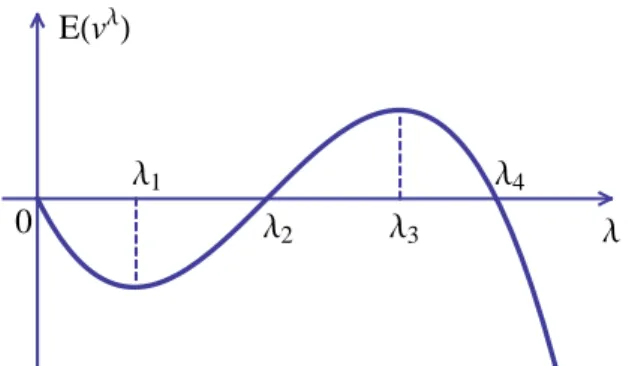
Lemma 1. If v ∈ H1(RN) satisfies E(v) > 0, then there exist λk = λk(v)
(k = 1, 2, 3, 4) such that 0 < λ1 < λ2 < λ3 < λ4 and
• E(vλ) is decreasing in (0, λ
1)∪ (λ3,∞), and increasing in (λ1, λ3).
• E(vλ) is negative in (0, λ
2)∪ (λ4,∞), and positive in (λ2, λ4).
• E(vλ) < E(vλ3) for all λ∈ (0, λ
3)∪ (λ3,∞).
Proof. Since a > 0, b > 0, 0 < α < 2 < β and E(v) > 0, the conclusion is
0 Λ1 Λ2 Λ3 Λ4 Λ EHvΛL
Figure 1: The graph of λ7→ E(vλ) for the case E(v) > 0.
Lemma 2. If v∈ H1(RN) satisfies E(v) > 0, Kω(v) < 0 and P (v) = 0, then d(ω) < Sω(v).
Proof. We consider two functions f (λ) = Kω(vλ) and g(λ) = E(vλ).
Since f (0) = ω∥v∥2L2 > 0 and f (1) = Kω(v) < 0, there exists λ0 ∈ (0, 1)
such that Kω(vλ0) = 0. Moreover, since vλ0 ̸= 0, it follows from (1.6) that d(ω)≤ Sω(vλ0).
On the other hand, since g′(1) = P (v) = 0 and g(1) = E(v) > 0, it follows from Lemma 1 that λ3= 1 and g(λ) < g(1) for all λ∈ (0, 1).
Thus, we have E(vλ0) < E(v), and
d(ω)≤ Sω(vλ0) = E(vλ0) + ω 2∥v λ0∥2 L2 < E(v) + ω 2∥v∥ 2 L2 = Sω(v).
This completes the proof.
Lemma 3. The setBωis invariant under the flow of (1.1). That is, if u0∈ Bω, then the solution u(t) of (1.1) with u(0) = u0 satisfies u(t) ∈ Bω for all t∈ [0, T∗).
Proof. Let u0 ∈ Bω and let u(t) be the solution of (1.1) with u(0) = u0. Then,
by the conservation laws (1.3), we have
0 < E(u(t)) = E(u0) < E(ϕω), ∥u(t)∥2L2 =∥u0∥2L2 =∥ϕω∥2L2 for all t∈ [0, T∗).
Next, we prove that Kω(u(t)) < 0 for all t∈ [0, T∗). Suppose that this were
not true. Then, since Kω(u0) < 0 and t7→ Kω(u(t)) is continuous on [0, T∗),
there exists t1 ∈ (0, T∗) such that Kω(u(t1)) = 0. Moreover, since u(t1) ̸= 0,
by (1.6), we have d(ω)≤ Sω(u(t1)). Thus, we have
d(ω)≤ Sω(u(t1)) = E(u0) + ω 2∥u0∥ 2 L2 < E(ϕω) + ω 2∥ϕω∥ 2 L2 = d(ω).
This is a contradiction. Therefore, Kω(u(t)) < 0 for all t∈ [0, T∗).
Finally, we prove that P (u(t)) < 0 for all t ∈ [0, T∗). Suppose that this were not true. Then, there exists t2 ∈ (0, T∗) such that P (u(t2)) = 0. Since
E(u(t2)) > 0 and Kω(u(t2)) < 0, it follows from Lemma 2 that d(ω) <
Sω(u(t2)). Thus, we have
d(ω) < Sω(u(t2)) = E(u0) + ω 2∥u0∥ 2 L2 < E(ϕω) + ω 2∥ϕω∥ 2 L2 = d(ω).
This is a contradiction. Therefore, P (u(t)) < 0 for all t∈ [0, T∗). Lemma 4. For any v∈ Bω,
E(ϕω)≤ E(v) − P (v).
Proof. Since Kω(v) < 0, as in the proof of Lemma 2, there exists λ0 ∈ (0, 1)
such that Sω(ϕω) = d(ω) ≤ Sω(vλ0). Moreover, since ∥vλ0∥2L2 = ∥v∥2L2 =
∥ϕω∥2L2, we have
(2.4) E(ϕω)≤ E(vλ0).
On the other hand, since P (vλ) = λ∂λE(vλ), P (v) < 0 and E(v) > 0, it
follows from Lemma 1 that λ3 < 1 < λ4. Moreover, since ∂λ2E(vλ) < 0 for
λ∈ [λ3,∞), by a Taylor expansion, we have
(2.5) E(vλ3)≤ E(v) + (λ
3− 1)P (v) ≤ E(v) − P (v).
Finally, by (2.4), (2.5) and the third property of Lemma 1, we have
E(ϕω)≤ E(vλ0)≤ E(vλ3)≤ E(v) − P (v).
This completes the proof.
Now we give the proof of Theorem 2.
Proof of Theorem 2. Let u0 ∈ Σ∩Bωand let u(t) be the solution of (1.1) with u(0) = u0. Then, by Lemma 3, u(t)∈ Bω for all t∈ [0, T∗).
Moreover, by the virial identity (1.8) and Lemma 4, we have 1
8
d2
dt2∥xu(t)∥ 2
L2 = P (u(t))≤ E(u(t)) − E(ϕω) = E(u0)− E(ϕω) < 0
§3. Proof of Theorem 1
First, we prove the following lemma.
Lemma 5. Let a > 0, b > 0, 1 < p < 1 + 4/N < q < 2∗− 1, and let ϕω∈ Gω. Then there exists ω1 > 0 such that E(ϕω) > 0 for all ω∈ (ω1,∞).
Proof. Since P (ϕω) = 0, we see that E(ϕω) > 0 if and only if
(3.1) (2− α)a p + 1 ∥ϕω∥ p+1 Lp+1 < (β− 2)b q + 1 ∥ϕω∥ q+1 Lq+1.
Moreover, in the same way as the proof of Theorem 2 in [13], we can prove that lim ω→∞ ∥ϕω∥p+1Lp+1 ∥ϕω∥q+1Lq+1 = 0.
Thus, there exists ω1 > 0 such that (3.1) holds for all ω∈ (ω1,∞).
Proof of Theorem 1. Let ω∈ (ω1,∞). Then, by Lemma 5, E(ϕω) > 0.
For λ > 0, we consider the scaling ϕλω(x) = λN/2ϕω(λx), and prove that
there exists λ0 ∈ (1, ∞) such that ϕλω∈ Bω for all λ∈ (1, λ0).
First, we have ∥ϕλω∥2L2 =∥ϕω∥2L2 for all λ > 0. Next, since P (ϕω) = 0 and E(ϕω) > 0, by Lemma 1 and (2.2), there exists λ4 > 1 such that
0 < E(ϕλω) < E(ϕω), P (ϕλω) < 0
for all λ∈ (1, λ4). Finally, since P (ϕω) = 0, we have ∂λKω(ϕλω) λ=1=− (p− 1)aα p + 1 ∥ϕω∥ p+1 Lp+1− (q− 1)bβ q + 1 ∥ϕω∥ q+1 Lq+1 < 0.
Since Kω(ϕω) = 0, there exists λ0 ∈ (1, λ4) such that Kω(ϕλω) < 0 for all λ∈ (1, λ0).
Therefore, ϕλ
ω ∈ Bω for all λ ∈ (1, λ0). Moreover, since ϕλω ∈ Σ for λ > 0,
it follows from Theorem 2 that for any λ∈ (1, λ0), the solution u(t) of (1.1)
with u(0) = ϕλω blows up in finite time. Finally, since lim
λ→1∥ϕ λ
ω− ϕω∥H1 = 0, the proof is completed.
Acknowledgment
The authors thank the referees for the careful reading of the manuscript. The research of the first author was supported in part by JSPS KAKENHI Grant Number 24540163.
References
[1] H. Berestycki and T. Cazenave, Instabilit´e des ´etats stationnaires dans les ´
equations de Schr¨odinger et de Klein-Gordon non lin´eaires, C. R. Acad. Sci. Paris S´er. I Math. 293 (1981), 489–492.
[2] H. Berestycki and P.-L. Lions, Nonlinear scalar field equations I, II, Arch. Ra-tional Mech. Anal. 82 (1983), 313–375.
[3] T. Cazenave, Semilinear Schr¨odinger equations, Courant Lect. Notes in Math., 10, New York University, Courant Institute of Mathematical Sciences, New York; Amer. Math. Soc., Providence, RI, 2003.
[4] T. Cazenave and P.-L. Lions, Orbital stability of standing waves for some non-linear Schr¨odinger equations, Comm. Math. Phys. 85 (1982), 549–561.
[5] R. Fukuizumi, Remarks on the stable standing waves for nonlinear Schr¨odinger equations with double power nonlinearity, Adv. Math. Sci. Appl. 13 (2003), 549– 564.
[6] R. Fukuizumi, M. Ohta and T. Ozawa, Nonlinear Schr¨odinger equation with a point defect, Ann. Inst. H. Poincar´e, Anal. Non Lin´eaire 25 (2008), 837–845. [7] J. Ginibre and G. Velo, On a class of nonlinear Schr¨odinger equations I. The
Cauchy problem, general case, J. Funct. Anal. 32 (1979), 1–32.
[8] T. Kato, On nonlinear Schr¨odinger equations, Ann. Inst. H. Poincar´e, Phys. Th´eor. 46 (1987), 113–129.
[9] S. Le Coz, A note on Berestycki-Cazenave’s classical instability result for non-linear Schr¨odinger equations, Adv. Nonlinear Stud. 8 (2008), 455–463.
[10] S. Le Coz, R. Fukuizumi, G. Fibich, B. Ksherim and Y. Sivan, Instability of bound states of a nonlinear Schr¨odinger equation with a Dirac potential, Phys. D 237 (2008), 1103–1128.
[11] M. Maeda, Stability and instability of standing waves for 1-dimensional nonlin-ear Schr¨odinger equation with multiple-power nonlinearity, Kodai Math. J. 31 (2008), 263–271.
[12] M. Ohta, Stability and instability of standing waves for one-dimensional non-linear Schr¨odinger equations with double power nonlinearity, Kodai Math. J. 18 (1995), 68–74.
[13] M. Ohta, Instability of standing waves for the generalized Davey-Stewartson sys-tem, Ann. Inst. H. Poincar´e, Phys. Th´eor. 62 (1995), 69–80.
[14] M. Ohta, Blow-up solutions and strong instability of standing waves for the gen-eralized Davey-Stewartson system in R2, Ann. Inst. H. Poincar´e, Phys. Th´eor. 63 (1995), 111–117.
[15] W. Strauss, Existence of solitary waves in higher dimensions, Comm. Math. Phys. 55 (1977), 149–162.
[16] J. Zhang, Cross-constrained variational problem and nonlinear Schr¨odinger equa-tion, Foundations of computational mathematics (Hong Kong, 2000), 457–469, World Sci. Publ., River Edge, NJ, 2002.
Masahito Ohta
Department of Mathematics, Tokyo University of Science 1-3 Kagurazaka, Shinjuku-ku, Tokyo 162-8601, Japan
E-mail : [email protected]
Takahiro Yamaguchi
Department of Mathematics, Tokyo University of Science 1-3 Kagurazaka, Shinjuku-ku, Tokyo 162-8601, Japan