A CONTINUOUS REVIEW INVENTORY MODEL WITH STOCHASTIC PRICES PROCURED IN THE SPOT MARKET

Vol. 53, No. 2, June 2010, pp. 136–148

A CONTINUOUS REVIEW INVENTORY MODEL WITH STOCHASTIC PRICES PROCURED IN THE SPOT MARKET

Kimitoshi Sato Katsushige Sawaki

Nanzan University

(Received August 28, 2009; Revised January 28, 2010)

Abstract Not only the amount of product demanded, but also the price of the product have a strong impact on a manufacturer’s revenue. In this paper we consider a continuous-time inventory model where the spot price of the product stochastically fluctuates according to a Brownian motion. Should information on the spot price be available, the manufacturer would wish to buy the product on the spot market when profitable. The purpose of this paper is to find an optimal procurement policy so as to minimize total expected discounted costs over an infinite planning horizon. We extend the Sulem (1986) model into one in which the market price of the product follows a geometric Brownian motion. By applying this, we obtain the optimal cost as a solution to a quasi-variational inequality, and show that there exists an optimal procurement solution as an (s,S) policy. We clarify the dependence of the optimal (s,S) policy on the spot price at the procurement epoch. These values of the (s,S) policy can be used and revised in the following ordering cycles. Finally, some numerical examples are provided to investigate the analytical properties of the expected cost function as well as of the optimal policy.

Keywords: Inventory, stochastic model, quasi-variational inequality

1. Introduction

Many manufacturers that use the spot market to procure parts and materials in their supply chains are face fluctuating market prices. In this paper we consider a continuous-time inventory model in which the spot price of the product fluctuates stochastically according to a Brownian motion. The inventory level can be monitored on a continuous time basis. Our objective is to determine the procurement policy as an (s,S) policy to reduce the risk of the spot price. When the inventory level drops down to the reorder point, a pair of order quantity and reorder points for the next cycle are determined based upon the observation of the spot price.

Price uncertainty has been taken into account by several researchers in the context of inventory policy. In a single-period model, Akella et al. [1] and Seifert et al. [14] develop a model that determines a combination of the optimal order quantity to purchase via forward contracts and the optimal quantity to purchase via spot markets in one a cycle period. The Seifert et al model allows the use of spot markets for both buying and selling. In a multi-period model, Goel and Gutierrez [9] consider the value of incorporating information about spot and futures market prices in procurement decision making. They use the two factor pricing model developed by Schwartz and Smith [13] to describe the stochastic evaluation of the commodity prices. Mart´ınez-deAlb´eniz and Simchi-Levi [11] address the dynamic supply contract selection problem of a manufacturer who can procure by using long-term and options contracts as well as the spot market.

Bather [3], Benkherouf and Aggoun [4], Benkherouf [5], Bensoussan et al. [7], Sulem [15] that are related to an (s,S) policy under continuous time review. Sulem [15] analyzes the optimal ordering policy by applying impulse control to an inventory system with stochastic demand followed by a diffusion process. Furthermore, Benkherouf [5] extends Sulem’s model to the case of general storage with a shortage penalty cost function. We also extend the Sulem model to the case in which the market price of the product follows geometric Brownian motions, but with deterministic demand.

The remainder of this paper is organized as follows. In section 2 we present the model formulation. It is shown in section 3 that the optimal cost can be derived as the solution to a quasi-variational inequality, and we show in section 4 that there exists an optimal procurement policy which is a type of an (s,S) policy. In section 5 we discuss the case of a specific type of spot price, and clarify the impact of the spot price on the value function. In Section 6, some numerical examples are provided to investigate the analytical properties of the expected cost function as well as of the optimal policy. Section 7 concludes the paper. 2. Notation and Assumptions

The analysis is based on the following assumptions:

(i) Time is continuous and inventory is continuously reviewed.

(ii) Demand is g units per unit time in one cycle. Unsatisfied demand is backlogged.

(iii) A critical-level (s, S, y) policy is in place, which means that the inventory level x drops to a reorder point s, then the inventory level increases up to S. And then the next s and

S are determined, based on the observation of the spot price y(t) at time t. Since s and S are changing at the beginning of each cycle, we define s and S to be the reorder point

and order-up-to level for the last cycle, respectively. Therefore, S represents the initial inventory level at the beginning of the next cycle (see Figure 1).

(iv) The set up cost is K and the unit cost is equal to the spot price y(·). The shortage cost

p and holding cost q are given by the function f : f (x) =

{

−px for x < 0,

qx for x≥ 0 (2.1)

where p and q satisfy the following conditions;

µy(t) > q, (2.2)

p + (µ− α)y(t) > 0. (2.3)

(v) The spot price at time t, y(t), follows a geometric Brownian motion, that is,

dy(t) = y(t)(µdt + σdw(t)) (2.4)

where w(t) follows a standard Brownian motion.

A procurement policy consists of a sequence V = {(θi, ξi), i = 1, 2,· · · } of i-th ordering

time θi and order quantity ξi. Let u(x, y) be the optimal total expected discounted cost

over an infinite planning horizon when an initial inventory level is given by x and the spot price by y. Then u(x, y) can be written as

u(x, y) = inf V ( E [∫ _∞ 0 f (x(t))e−αtdt +∑ i≥1 (K + y(θi)ξi)e−αθi ¯¯ ¯¯x(0) = x,y(0) = y ]) (2.5)

x S s S s τx τ_S Inventory Time Spot price y y

Figure 1: Inventory flow

where the inventory level x(t) is given by

dx(t) =−gdt +∑ i≥1

ξiδ(t− θi) (2.6)

with x(0) = x and α being the discount rate. Here, we assume that α ≥ µ > 0. In equation (2.6), δ(·) denotes the Dirac function, that is,

δ(z) =

{

1 for z = 0,

0 otherwise. (2.7)

Here, we assume that u(x, y) is continuous and everywhere differentiable in x, and also that it is twice differentiable in y. Although this assumption is not mathematically rigorous, the theory of viscosity solutions [8] ensures that value function u is always characterized as a generalized solution of the associated partial differential problem in some weak sense and is uniquely determined.

Our objective is to find the optimal procurement policy (s,S) at which the minimum value function u will be attained．

3. The QVI Problem and Optimal Procurement Policy

In this section, we deal with equation (2.5) as a Quasi-Variational Inequality (QVI) problem (Bensoussan and Lions [6]).

First, if the procurement is not made at least during the small time interval (t, t + ²), then we have following inequality:

u(x(t), y(t)) ≤

∫ t+² t

f (x(s))e−α(s−t)ds + u(x(t + ²), y(t + ²))e−α². (3.1) If expand the right-hand side of equation (3.1) up to the first order in ², then we have

²f (x) + u(x, y)− g²∂u ∂x + µy² ∂u ∂y + 1 2²σ 2 y2∂ 2_u

∂y2 − α²u(x, y) + o(² 2

Hence, letting ² trend to 0, equation (3.1) can be reduced to 1 2σ 2_y2∂2u ∂y2 + µy ∂u ∂y − g ∂u ∂x − αu ≥ −f(x). (3.3)

On the other hand, if the procurement is made at time t, the inventory level jumps from

x to an x + ξ. We assume that the order quantity is delivered immediately, so the spot price

before the procurement is equal to the price after procurement. Thus, we obtain

u(x, y)≤ K + inf

ξ≥0(y(t)ξ + u(x + ξ, y(t))). (3.4)

Since we make a decision to minimize the expected total cost, at least one of inequalities (3.3) and (3.4) must hold as an equality. Therefore, equation (2.5) is resolved by a solution to the QVI problem:

min(Au + f, M u− u) = 0, (3.5) where Au(x, y) := 1 2σ 2_y2∂2u ∂y2 + µy ∂u ∂y − g ∂u ∂x − αu, (3.6) M u(x, y) := K + inf

ξ≥0(y(t)ξ + u(x + ξ, y(t))). (3.7) 4. The Solution of the QVI Problem

In this section, we partially solve the QVI problem (3.5) from Sulem [15]. We divide the inventory space into two regions; for no procurement,

G ={x ∈ R : u(x, y) < Mu(x, y)} = {x ∈ R : x > s} (4.1) then, we have

Au + f = 0. (4.2)

And its complement is given by

G ={x ∈ R : u(x, y) = Mu(x, y)} = {x ∈ R : x ≤ s} (4.3)

and for x∈ G, we have

u(x, y) = K + inf

ξ≥0(y(t)ξ + u(x + ξ, y(t))) (4.4)

= K + y(t)(S− x) + u(S, y(t)). (4.5)

Due to deterministic demand, we take the inventory level within the elapsed time from the beginning of the cycle. Thus, we describe the spot price with yx when the inventory

level is x hereafter.

Since u is continuously differentiable in x, in inventory space G, we can get the boundary conditions on u.

(i) Continuity of the derivative of u at the boundary point s: lim

x↓s

∂u(x, y)

(ii) The infimum in equation (4.4) is attained at S: lim

x↑S

∂u(x, y)

∂x =−y, (4.7)

where y is the spot price at the beginning of the cycle. (iii) u is continuous at s:

u(S, y) = u(s, y)− K − ys(S− s). (4.8)

(iv) The growth condition of u:

lim

x→∞

u(x, y)

f (x) < +∞. (4.9)

To obtain the value function u, we solve the partial differential equation (4.2) with the initial and boundary conditions (4.6)-(4.8). First, we set

u(x, y) = w(τ, z)ekz+lτ, z = log y, τ = x− s

g . (4.10)

Then, equation (4.2) can be rewritten as follows; ( l− µk + α +1 2k(1− k)σ 2 ) w +∂w ∂τ + (( 1 2− k ) σ2− µ ) ∂w ∂z − σ2 2 ∂2_w ∂z2 = f (gτ + s)e −(kz+lτ)_{. (4.11)}

By choosing k and l to satisfy

k =− 1 σ2 ( µ− 1 2σ 2 ) , l =− 1 2σ2 ( µ− 1 2σ 2 )2 − α, (4.12)

we can get the non-homogeneous heat equation

∂w ∂τ − σ2 2 ∂2_w ∂z2 = f (gτ + s) exp { 1 σ2 ( µ− 1 2σ 2 ) z + ( 1 2σ2 ( µ− 1 2σ 2 )2 + α ) τ } (4.13) with w(0, z) = eσ21 “ µ−σ2 2 ” z {v(τS, z) + K + ez(S− s)} ≡ m(z), (4.14) τS = S− s g . (4.15)

The solution to the diffusion equation problem is given by

w(τ, z) = w1(τ, z) + w2(τ, z), (4.16)

where w1(τ, z) and w2(τ, z) are solutions to the following problems:

∂w1 ∂τ = σ2 2 ∂2w1 ∂z2 , w1(0, z) = m(z), (4.17) ∂w2 ∂τ = σ2 2 ∂2_w 2 ∂z2 + h(τ, z), w2(0, z) = 0. (4.18)

Here, we set the right hand side of equation (4.13) as h(τ, z). The solutions w1, w2 of problems (4.17) and (4.18) are, respectively, given by

w1(τ, z) = 1 √ 2πσ2_τ ∫ _∞ −∞ w1(0, ξ) exp { −(z− ξ)2 2σ2_τ } dξ = √1 2πe n−(τ,z) ∫ _∞ −∞ v ( τS, τ ( µ− σ 2 2 ) + λσ√τ + z ) e−λ22 dλ +Ken−(τ,z)_{+ (S− s)e}n+(τ,z)_{, (4.19)} and w2(τ, z) = 1 √ 2πσ2 ∫ τ 0 1 √ τ − δ ∫ _∞ −∞ h(δ, ξ) exp ( − (z− ξ)2 2σ2_(τ − δ) ) dξdδ = en−(τ,z) ∫ τ 0 f (gδ + s)eαδdδ, (4.20) where n_±(τ, z) = 1 2σ2 ( µ± σ 2 2 ) ( τ ( µ± σ 2 2 ) + 2z ) . (4.21)

Therefore, from equations (4.10), (4.16), (4.19) and (4.20), u(x, y) can be rewritten as follows; u(x, y) = e−ατx [ 1 √ 2π ∫ _∞ −∞ u(S, yxe τx “ µ−σ2 2 ” +λσ√τx )e−λ22 dλ +K + (S− s)yxeµτx + ∫ τx 0 f (gδ + s)eαδdδ ] . (4.22)

The last term of equation (4.22), it can be rewritten as

D(x) ≡ ∫ τx 0 f (gδ + s)eαδdδ = { p α ( s−_αg)+ _αq (x− _αg)eατx ₊ g α2(p + q)e− α gs for x≥ 0, −p α {( x−_αg)eατx− s + g α } for x < 0, (4.23) and D(s) = 0. Therefore, we have

u(x, y) = e−ατx_{[E[u(S, y} xeτx(µ− σ2 2 )+σ √_τ xX_{)] + K + (S}− s)y xeµτx + D(x)] = e−ατx_{[u(S, y) + K + (S}− s)y xeµτx + D(x)] (4.24)

where X is a standard normal random variable.

Lemma 1. The optimal cost function u(x, y) is given by

u(x, y) = g α ( q gS + y ) eα(τS−τx)₊ { yxe(µ−α)τx− ( 1− µ α ) yeµτS−ατx } (S− s) + L(x) (4.25) where L(x) = { q α {( x−_αg)−(S−_αg)eα(τ_S−τx)} _{for x}≥ 0, −p α ( x− _αg)− _αq (S−_αg)eα(τ_S−τx)− g α2(p + q)e− α gx _{for x < 0.} (4.26)

Proof. By equations (4.7) and (4.24), we have u(S, y) = g α ( q gS + y ) eατS − ( 1− µ α ) (S− s)yeµτS − K − D(S). (4.27)

Thus, equations (4.24) and (4.27) lead to equation (4.25).

Remark 1. Note that equation (4.25) can be reduced to the deterministic-demand case of Sulem’s model when we assume µ = σ = 0, y = y and S = S. In this case, the optimal cost ˜

u(x) can be reduced to be

˜ u(x) = { (q + αy)g α2 e αS g − qg α2 } e−αxg + r αx + rg α2 ( e−αxg − 1 ) (4.28) where r = { −p for x < 0, q for x≥ 0. (4.29) Proposition 1. If yx ≥ (

1− µ_α)yeµ(τ_S−τx)_{, then u(x, y)}≥ ˜u(x) for all x and y.

Proof. Subtracting equation (4.28) from equation (4.25), we get u(x, y)− ˜u(x) = { yxe(µ−α)τx − ( 1− µ α ) yeµτS−ατx } (S− s) (4.30)

for all x. Hence, we have u(x, y)≥ ˜u(x) for yx ≥

( 1−_αµ)yeµ(τ_S−τx)_. Lemma 2. If µ satisfies α + 1 τS log ( 1− q µyx ) < µ ≤ α, (4.31)

and there exists an optimal order point s for any y, then s is strictly negative. Proof. From equation (4.25), we have

∂u ∂y = e

(µ−α)τx_(S− s), ∂ 2_u

∂y2 = 0. (4.32)

Therefore, Au + f = 0 can be rewritten as

−µyxe(µ−α)τx(S− s) + g ∂u

∂x + αu = f (x). (4.33)

Here, we assume that s≥ 0 and we can obtain

∂u(S, y)

∂x =−ys (4.34)

from the same type of reasoning that gave equation (4.7). It follows from equations (4.33) and (4.34) that

αu(S, y) = qS + gys+ µyse(µ−α)τS(S− s) as x → S (4.35)

and from (4.6) that

αu(s, y) = qs + gys+ µys(S− s) as x → s. (4.36) Hence, s < S and α +_τ1 S log ( 1− _µyq s )

< µ≤ α yield the result that u(S, y) > u(s, y). This

Next we explore the properties of u and demonstrate the existence of an optimal policy based on Benkherouf [5]. Let us denote H(x, y) = u(x, y) + yxx. Then, equation (4.2) can

be rewritten as

g∂H

∂x + αH = gyx+ αyxx + f (x) + µyxe

(µ−α)τx_(S− s). _(4.37)

Lemma 3. Assume that equation (4.31) holds. Then, there exists a pair (s,S) such that s

and S satisfy equations (4.6)-(4.8).

Proof. It suffices to show that H(s, y) < K + H(S, y) for s→ 0, and H(s, y) > K + H(S, y)

for s→ −∞. For s → 0 in equations (4.35) and (4.36), we get

u(S, y)− u(s, y) = S

α(q + µys(e

S

g(µ−α)− 1)) _(4.38)

Hence, by assumption (4.31), we have u(S, y) > u(s, y) which implies that

H(s, y) = u(s, y) + sy < u(S, y) + Sy + K = H(S, y) + K. (4.39) Next, we show that H(s, y) > K + H(S, y) for s→ −∞. It follows from equation (4.25) that H(s, y) = g α2 ( (αy + q)eαgS− (p + q) ) e−αgs− p α ( s− g α ) + ysS− ( 1− µ α ) yeµτS(S− s). (4.40) For µ≤ α, applying l’Hospital’s rule to equation (4.40), we have

g α2 ( (αy + q)eαgS− (p + q) ) e−αgs− p α ( s− g α ) ≈ −p α ( s− g α ) → +∞ (4.41) as s→ −∞, and −(1− µ α ) yeµτS(S− s) ≈ − g αµ(µ− α)ye µτ_{S =}      +∞ for 0 < µ < α, 0 for µ = α, − g αµ(µ− α)y for µ ≤ 0. (4.42)

Thus, H(s, y) → +∞ as s → −∞ for µ ≤ α. Also, we have H(x, y) → +∞ as x → +∞. Consequently, there exists an S such that ∂H(S,y)_∂x = 0 and H(s, y) > K + H(S, y) as

s→ −∞.

Lemma 4. If (s,S) is the solution of a QVI problem (3.5), then we have ∂H(x, y)/∂x≤ 0

if s≤ x ≤ S, and ∂H(x, y)/∂x ≥ 0 if S ≤ x for any y.

Proof. First, we show that ∂H(x, y)/∂x≤ 0 for s ≤ x ≤ S. Suppose that ∂H(x, y)/∂x > 0.

In terms of equation (4.8), we have H(S, y) < H(s, y), which is in contradiction with

∂H(x, y)/∂x > 0.

Next, we show that ∂H(x, y)/∂x≥ 0 for S ≤ x. Assume that ∂H(x, y)/∂x ≤ 0 for S ≤ x. From H(x, y) decreases for s≤ x ≤ S and H(x, y) → +∞ as x → +∞, there exists a number

S < ˜S, such that ∂H( ˜S, y)/∂x = 0, ∂2_{H( ˜S, y)/∂x}2 _{≥ 0 and H(S, y) > H( ˜S, y). Therefore,} we have ∂H(x, y)/∂x ≥ 0 for ˜S ≤ x, and it is in contradiction with ∂H(x, y)/∂x ≤ 0 for S ≤ x. This completes the proof.

Theorem 1. Under assumptions (2.2), (2.3) and (4.31), the optimal policy (s,S) is a unique solution to the QVI problem, and the value of (s,S) is given by the solution of the following simultaneous equations:

g α ( p gs− ys ) + q α ( S− g α ) + g α ( y + q α ) eα(τS−τS)_{+ K} + { yse(µ−α)τS + ( 1− µ α ) (ys− yeµτS−ατS) } (S− s) = 0 (4.43) g α ( q gS + y ) eατS − q α ( S− g α ) − g α ( y + q α ) eα(τS−τS)− D(S) − K −{yse(µ−α)τS + yeµτS ( 1− µ α ) (1− e−ατS₎ } (S− s) = 0 (4.44)

Proof. Equations (4.43) and (4.44) are derived from equations (4.6) and (4.8). First, we

show the QVI relations (3.5), that is, Au + f ≥ 0 for x ≤ s and u ≤ Mu for x ≥ s. For

x≤ s, we obtain following equation by using equation (4.8);

u(x, y) = u(s, y) + yx(S− x) − ys(S− s). (4.45)

Then, Au + f ≥ 0 can be rewritten as

αu(s, y)− αys(S− s) ≤ f(x) + gyx− (α − µ)yx(S− x). (4.46)

Therefore, it is only necessary to show that C(x)≥ 0 for x ≤ s, where

C(x) ≡ f(x) + gyx− (α − µ)yx(S− x) − αu(s, y) + αys(S− s). (4.47)

Taking the derivative of C(x), we have C0(x) = −p − (µ − α)yx < 0 from condition (2.3).

This implies that C(x) is decreasing for x≤ s. From Au + f = 0, we have

C(s) = f (s) + gys− (α − µ)ys(S− s) − αu(s, y) + αys(S− s) = 0. (4.48)

Thus, C(x)≥ 0 for x ≤ s.

Next, we show that u ≤ Mu for x ≥ s. For s ≤ x ≤ S, we have

M u(x, y) = K + yx(S− x) + u(S, y) (4.49)

which implies

M u(x, y)− u(x, y) = −H(x, y) + K + yxS + u(S, y). (4.50)

Differentiating the above equation with respect to x, then we get

∂

∂x[M u(x, y)− u(x, y)] = −

∂H(x, y)

∂x . (4.51)

As x → s in equation (4.49), we have Mu = u. Also, we have Mu − u = K as x → S in equation (4.50). Since ∂H(x,y)_∂x ≤ 0 for s ≤ x ≤ S, we obtain u ≤ Mu for s ≤ x ≤ S from equation (4.51). Finally, for x ≥ S, we have Mu(x, y) = K + u(x, y). It clearly holds for

Second, we show that (s,S) is a unique solution to the QVI problem. Suppose that there are two solutions (s1,S1) and (s2,S2) with s1 < s2 and S2 < S1. This means that

∂H(s1,y)

∂x =

∂H(s2,y)

∂x = 0. Thus, there exists at least one x∗ ∈ (s1, s2) such that

∂2_H(x∗_,y)

∂x = 0

and ∂H(x_∂x∗,y) < 0.

For x∗ < s2, we have Au(x∗, y) + f (x∗)≥ 0, that is,

αH(x∗, y)≤ αyx∗x∗+ gyx∗+ µyx∗(S2− x∗)− px∗. (4.52) On the other hand, we get Au(x∗, y) + f (x∗) = 0 from s1 < x∗,

g∂H(x ∗_{, y)}

∂x + αH(x

∗_{, y) = gy}

x∗ + αyx∗x∗ − px∗+ µyx∗e(µ−α)τx∗(S1− s1). (4.53)

Thus, equations (4.52) and (4.53) lead to

∂H(x∗, y) ∂x ≥ µ gyx∗(e (µ−α)τx∗_(S 1− s1)− (S2− x∗)). (4.54)

We can see that∂H(x_∂x∗,y) ≥ 0 from equation (4.54), which is in contradiction with ∂H(x_∂x∗,y) < 0.

Thus, we have the required result.

Remark 2. When the drift of the spot price µ is equal to the discount rate α, then the simultaneous equation (4.43)-(4.44) becomes the simple form:

s = 1 αys− p [ g ( y + q α ) eα(τS−τS)− g ( ys+ q α ) + (q + αys)S + αK ] (4.55) g α ( q gS + y ) eατS− q α ( S− g α ) − g α ( y + q α ) eα(τS−τS)− D(S) − K − y_s(S− s) = 0 (4.56) 5. Specific Spot Price Types

Since equations (4.43) and (4.44) depend on the spot price ys at the end of the cycle, we

assume that the price is equal to the expectation of the spot price at the end of the cycle in order to estimate the total cost at the beginning of cycle. Thus, we assign

yx = yeµ(τS−τx) (5.1)

to equation (4.25).

Then, the value function u is as follows;

u(x) = g α ( q gS + y ) eα(τS−τx)+ µ αye µτ_S−ατx_(S− s) + L(x) _(5.2)

where L(x) is given by equation (4.26).

Proposition 2. u(x) is increasing in y and µ.

Proof. From equation (5.2), we get ∂u ∂y = g αe α(τ_S−τx) { 1 + µ ge (µ−α)τ_{S(S− s)} } > 0, (5.3) ∂u ∂µ = 1 αye µτ_S−ατx_(S− s) ( 1 + µS− s g ) > 0. (5.4)

We recalculate equations (4.43) and (4.44) to implement numerical computing. Then we have p gs + q g ( S− g α ) + α gK− ye µτ_{S +}(_{y +} q α ) eα(τS−τS) y g { α(1 + (eµτS − 1)(eµτS−ατS _{+ 1)) + µe}µτS−ατS}_(S− s) = 0, (5.5) −(y + q α ) (1− e−ατS_)eατS +p g ( s− g α ) + q g ( S− g α ) + 1 α(p + q)e −α gs+α gK y g { α(1 + (eµτS − 1)(eµτS−ατS _{+ 1))}− µeµτS(1− e−ατS₎}_(S− s) = 0. (5.6) 6. Numerical Examples

In this section we present a numerical example of optimal procurement policy using equa-tions (5.5) and (5.6), and illustrate its value function. We assume that g = 0.2, p = 0.2,

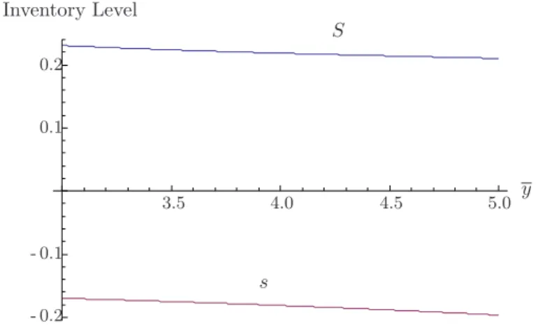
q = 0.04, K = 0.14, α = 0.02, µ = 0.015, σ = 0.12, y = 3.0 and S = 0.586. Then, we have S = 0.231, s =−0.17. Figure 2 shows the optimal cost function u and ˜u that the optimal

cost for the spot price model is higher than Sulem’s result for the fluctuation of the spot price. By proposition 1, we know that the property holds. Figure 3 expresses the relation-ship between the optimal policy and the drift parameter. Moreover, Figure 4 illustrates the optimal policy with respect to the initial spot price. We can see that the reorder point s increases and S decreases for µ in Figure 3. Comparing Figure 3 with Figure 4, we find that the order quantity is highly sensitive to the drift parameter of the spot price.

- 5 0 5 10 15 20 25 30 20 30 40 50 u ˜ u x Optimal Total Cost

0.005 0.010 0.015 0.020 - 0.4 - 0.2 0.2 0.4 Inventory Level S s µ

Figure 3: The optimal procurement policy with respect to µ

3.5 4.0 4.5 5.0 - 0.2 - 0.1 0.1 0.2 y Inventory Level S s

Figure 4: The optimal procurement policy with respect to y

7. Concluding Remarks and Further Research

In this paper, we showed the existence of an optimal policy for the inventory model that permits manufacturers to procure products from the spot market. We obtained the optimal cost function as a solution of a quasi-variational inequality, and showed that there exists an optimal procurement policy which is described by the form of an (s,S) policy. For future research, we may extend the inventory model of procurement from spot market into a model where demand also follows a diffusion process and incorporates supply contracts like options or futures.

8. Acknowledgment

The authors wish to thank to anonymous referees for their many helpful comments which make the paper much more readable. This research has received a financial aids from the Grant-in-Aid for Science Research (No. 20241037) of the Japanese Society of the Promotion of Science in 2008-2012.

References

[1] R. Akella, V. Araman and J. Kleinknecht: B2B Markets: Procurement and Supplier Risk Management. In J. Geunes, H. E. Romeijin and P. Kouvelis (eds.): Supply Chain

Management-Applications and Algorithms (Kluwer Academic Publishers, 2002).

[2] A. Bar-Ilan and A. Sulem: Explicit solution of inventory problems with delivery lags.

Mathematics of Operations Research, 20 (1995), 709–720.

[3] J.A. Bather: A continuous time inventory model. Journal of Applied Probability, 3 (1966), 538–549.

[4] L. Benkherouf and L. Aggoun: On a stochastic inventory model with deterioration and stock-dependent demand items. Probability in the Engineering and Informational

Sciences, 16 (2002), 151–165.

[5] L. Benkherouf: On a stochastic inventory model with a generalized holding costs.

European Journal of Operational Research, 182 (2007), 730–737.

[6] A. Bensoussan and J.L. Lions: Impulse Control and Quasi-variational Inequalities (Gauthier Villars, Paris, 1984).

[7] A. Bensoussan, R.H. Liu, and S.P. Sethi: Optimality of an (s, S) policy with com-pound Poisson and diffusion demands: a quasi-variational inequalities approach. SIAM

Journal on Control and Optimization, 44 (2005), 1650–1676.

[8] M.G. Crandall, H. Ishii and P.L. Lions: User’s guide to viscosity solutions of second order partial differential equations. Bulletin of the American Mathematical Society, 27 (1992), 1–67.

[9] A. Goel, and G.J. Gutierrez: Integrating spot and futures commodity markets in the optimal procurement policy of an assembly-to-order manufacturer. working paper, Man-agement Department, University of Texas, Austin, (2004).

[10] X. Guo, P. Tomecek and M. Yuen: Optimal spot market inventory strategies in the presence of cost and price risk. working paper, University of California, Berkeley, (2007). [11] V. Mart´ınez-deAlb´eniz and D. Simchi-Levi: A portfolio approach to procurement

con-tracts. Production and Operations Management, 14 (2005), 90–114.

[12] P.V. O’Neil: Beginning Partial Differential Equations (John Wiley and Sons, New York, 1999).

[13] E.S. Schwartz and J.E. Smith: Short-term variations and long-term dynamics in com-modity prices. Management Science, 46 (2000), 893–911.

[14] R.W. Seifert, U.W. Thonemann and W.H. Hausman: Optimal procurement strategies for online spot markets. European Journal of Operational Research, 152 (2004), 781– 799.

[15] A. Sulem: A solvable-one dimensional model of a diffusion inventory system.

Mathe-matics of Operations Research, 11 (1986), 125–133.

Kimitoshi Sato

Graduate School of Business Administration, Nanzan University

Research Fellow of the Japan Society for the Promotion of Science,

18 Yamazato-cho, Showa-ku, Nagoya 466-8673, Japan