パターン認識のための表現学習法の考察と拡張

パターン認識のための表現学習法の考察と拡張

イワナ, ブライアン ケンジ

https://doi.org/10.15017/1931934

出版情報：Kyushu University, 2017, 博士（学術）, 課程博士 バージョン：

権利関係：

for Pattern Recognition

Brian Kenji Iwana

Department of Advanced Information Technology Doctor of Philosophy

KYUSHU UNIVERSITY

February 2018

Extension and Inspection of Representation Learning for Pattern Recognition

Brian Kenji Iwana

Department of Advanced Information Technology February 2018

Doctor of Philosophy

Abstract

There is a question in machine learning of how to use representation and feature learning to develop effective models for pattern recognition. This thesis proposes two methods of efficient time series recognition. The first model proposes the use of Dynamic Time Warping (DTW) as a distance measure for time series to embed dissimilarities into vector space using Dissimilarity Space Embedding (DSE). Next, the thesis introduces the idea of using AdaBoost as a prototype selection and ensemble classifier building solution to reduce the dimensionality of the space created by DSE.

For the second method, a novel feed forward network for time series called a Dynamic

Time Warping Neural Network (DTW-NN) is proposed. DTW-NNs implement DTW

as a kernel-like function and integrate them into fully-connected neural networks by

replacing the traditional linear kernel. In addition, this thesis explores the internal

representations learned by Convolutional Neural Networks (CNN). CNNs typically

are trained on large quantities of data, but often times acquiring heavily annotated

supervised labels for object detection is difficult. However, the thesis shows that it is

possible for CNNs to develop inferred representations of image components with only

image-level labels. This thesis also explores the internal representations and describes

the characteristics of correctly detected components.

Acknowledgments

I would like to thank my supervisor, Prof. Seiichi Uchida, for his guidance and the

opportunity to be part of his wonderful lab. In addition, I would like to thank my

committee members, Prof. Taniguchi and Prof. Shimada for their interest and their

help with the supervision of this thesis. I am also grateful for my colleagues and

co-authors which have provided valuable advice and meaningful contributions to my

work, some of which includes Dr. Volkmar Frinken, Dr. Kaspar Riesen, Letao Zhou,

Prof. Kumiko Tanaka-Ishii, Kotaro Abe, Shota Ide, Dr. Anna Zhu, Jinho Lee, Syed

Tahseen Raza Rizvi, Dr. Sheraz Ahmed, and Prof. Andreas Dengel. I would like to

thank all of the members of the Human Interface Laboratory, past and present, that

have provided me with friendship and stability. In addition, I would like to thank the

Institute of Decision Science for a Sustainable Society and the professors that have

helped me along the way. Finally, I would like to thank my family and Yirong Zhao

for the love and support that they have given me.

1 Introduction 17

1.1 Motivation . . . . 19

1.1.1 Effectiveness . . . . 19

1.1.2 Efficiency . . . . 20

1.2 Purpose . . . . 21

1.2.1 Extending Dissimilarity Representation . . . . 21

1.2.2 Extending Deep Learning Representation . . . . 21

1.2.3 Inspecting Representation Learning . . . . 22

1.3 Contributions . . . . 23

1.4 Organization of Thesis . . . . 25

I Representation Learning for Time Series 26 2 Background 27 2.1 Time Series Recognition . . . . 27

2.1.1 Example: Online Handwritten Character Recognition . . . . . 28

2.1.2 Dynamic Time Warping (DTW) . . . . 30

2.2 Dissimilarity Representation . . . . 37

2.2.1 Dissimilarity Space Embedding (DSE) . . . . 37

2.2.2 Prototype Selection for DSE . . . . 38

2.3 Deep Learning Representation . . . . 43

7

2.3.1 Artificial Neural Networks (ANN) . . . . 44

2.3.2 Feed Forward Neural Networks . . . . 44

2.3.3 Feed Forward Neural Networks for Time Series . . . . 51

2.3.4 Recurrent Neural Networks (RNN) . . . . 53

2.4 Summary . . . . 54

3 Ensemble Method for Dissimilarity Representations 57 3.1 DTW Distance Based DSE . . . . 57

3.2 DSE with AdaBoost for Prototype Selection . . . . 58

3.2.1 AdaBoost . . . . 59

3.2.2 DSE with AdaBoost . . . . 61

3.3 Experiment Setup . . . . 62

3.3.1 Dataset Preparation . . . . 62

3.3.2 Comparative Methods . . . . 63

3.4 Results . . . . 65

3.5 Discussion . . . . 67

3.5.1 Efficiency of Prototype Reduction . . . . 67

3.5.2 What Makes a Good Prototype for DSE? . . . . 69

3.5.3 On Using External Class Prototypes . . . . 70

3.5.4 Discriminability of AdaBoost Selected Prototypes . . . . 75

3.5.5 Comparison to Other DSE Prototype Selection Methods . . . 75

3.6 Summary . . . . 78

4 Dynamic Alignment for Deep Learning Representations 81 4.1 Dynamic Time Warpring Neural Networks (DTW-NN) . . . . 82

4.1.1 DTW as a Nonlinear Inner Product . . . . 83

4.1.2 Formulation of a DTW Layer . . . . 85

4.2 Representation Learning through DTW-NN . . . . 91

4.3 Experiment Setup . . . . 91

4.3.1 Dataset Preparation . . . . 92

4.3.2 Hyperparameters and Architecture Settings . . . . 92

4.3.3 Comparative Methods . . . . 93

4.4 Results . . . . 95

4.5 Discussion . . . . 95

4.5.1 Hyperparameters and Initialization . . . . 95

4.5.2 Analysis of the Weights . . . . 98

4.5.3 Comparison of DTW-NN to Baseline Methods . . . 102

4.6 Summary . . . 104

II Representation Learning for Images 107 5 Background 109 5.1 Image Recognition . . . 109

5.1.1 Example: Chinese Character Component Awareness . . . 109

5.2 Deep Learning Representation . . . 115

5.2.1 Convolutional Neural Networks (CNN) . . . 115

5.2.2 Object Detection with CNNs . . . 118

5.3 Summary . . . 120

6 Understanding Deep Learning Representations 123 6.1 Component Awareness with CNNs . . . 123

6.2 Experiment Setup . . . 124

6.2.1 Dataset Preparation . . . 124

6.2.2 Hyperparameters and Architecture Settings . . . 125

6.2.3 Evaluation Metrics . . . 125

6.3 Results . . . 126

6.4 Discussion . . . 128

6.4.1 Factors Contributing to Component Detection . . . 128

6.4.2 Effects of Component Removal . . . 131 6.5 Summary . . . 133

7 Conclusion 135

A Prototypes Selected by DSE with AdaBoost 139

B Prototypes Selected by DSE with AdaBoost + External Classes 149

C Confusion Matrices of DTW-NN and LSTM 159

1-1 Flowchart comparing representation learning to classic methods . . . 18

2-1 Example of a time series with temporal distortions . . . . 28

2-2 Examples from the Unipen dataset . . . . 29

2-3 Comparison between linear matching and dynamic matching . . . . . 30

2-4 Demonstration of a DTW calculation . . . . 32

2-5 DTW slope constraints . . . . 34

2-6 Global constraints of DTW . . . . 35

2-7 Comparison of linearly matched distances and DTW distances . . . . 36

2-8 Visualization of DSE . . . . 38

2-9 Illustration of an MLP . . . . 45

2-10 Illustration of a TDNN . . . . 52

2-11 Illustration of a WaveNet . . . . 53

2-12 Illustration of an RNN . . . . 54

2-13 Illustration of an LSTM . . . . 55

3-1 DTW-based DSE . . . . 58

3-2 DSE with AdaBoost . . . . 61

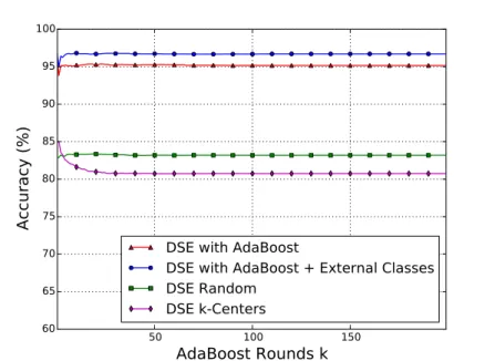
3-3 Comparative accuracy for DSE with AdaBoost . . . . 67

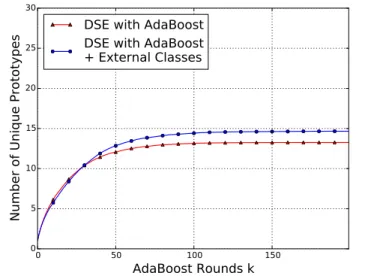
3-4 Prototype reduction from AdaBoost . . . . 68

3-5 Prototypes selected by DSE with AdaBoost for “0” and “6” . . . . 69

3-6 Histograms of good versus bad dissimilarity distributions . . . . 69

11

3-7 Example of the benefit of using external classes in DSE . . . . 70

3-8 External class usage for DSE with AdaBoost + External Class . . . . 72

3-9 Prototypes selected by DSE with AdaBoost + External Classes for “0” and “6” . . . . 73

3-10 Variations of class “5” . . . . 73

3-11 DSE comparisons for “5” and “8” . . . . 74

3-12 Prototypes selected by DSE with AdaBoost + External Classes for “5” and “8” . . . . 75

3-13 Comparative accuracy of 1-NN with prototype selection . . . . 76

3-14 Example of 𝑘 -Centers prototype selection . . . . 77

4-1 MLP node with temporal distortion . . . . 82

4-2 Comparison of a dot product and DTW . . . . 83

4-3 Illustration of a DTW-NN . . . . 86

4-4 DTW node with temporal distortion . . . . 87

4-5 Effect of learning rate on DTW-NN . . . . 97

4-6 Effect of weight initialization on DTW-NN . . . . 98

4-7 Progression of weights from a DTW node . . . . 99

4-8 The weights of DTW nodes after training . . . 100

4-9 t-SNE of DTW node activations through training . . . 101

4-10 Comparison of the misclassifications of “b” . . . 103

4-11 The misclassifications of “o” of the LSTM . . . 104

4-12 Comparison of the misclassifications of “t” . . . 104

5-1 Examples of Chinese characters with their components highlighted . . 113

5-2 Decomposition of a Chinese character . . . 113

5-3 Illustration of a CNN . . . 116

5-4 Demonstration of max pooling . . . 118

5-5 Examples of supervision for detection . . . 120

6-1 Example results for the component “

” . . . 128

6-2 Example results for the component “

” . . . 129

6-3 Example results for the component “亻” . . . 130

6-4 Example results with the component “

2.1 Common Activation Functions for ANNs . . . . 47

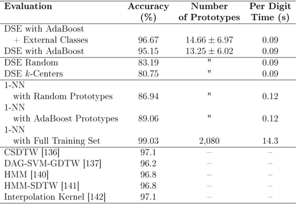
3.1 Comparative Accuracies for DTW-based DSE with AdaBoost for the Unipen 1a Dataset. . . . 66

4.1 Comparative Accuracies (%) for DTW-NN . . . . 95

4.2 Accuracies for DTW-NN at Different Learning Rates . . . . 96

5.1 Chinese Compound Character Structures . . . 112

6.1 Chinese Character Component Detection Results . . . 127

6.2 Chinese Character Component Detection Results with Component Re- moved . . . 132

15

Introduction

Pattern recognition is a branch of study that aims to find patterns in data and to understand its attributes [1]. In particular, pattern classification assigns labels, or classes, to data. Pattern recognition and classification are essential for understanding the real world and can be traced back to the beginning of human evolution and cognition [2]. It is thoroughly intertwined in daily life and machine-based pattern recognition aims to solve a wide array of applications with the use of computers. For example, some of these applications include, object detection and recognition, text recognition, handwriting and speech recognition, action and gesture analysis, and more.

In the past, pattern recognition algorithms used rule-based systems which im- plement hand-designed programs for decision making. However, these methods are inflexible and cannot be generalized to applications they were not designed for. Fol- lowing rule-based systems, early machine learning methods employed more general models which could learn from predetermined features. Using machine learning was a large step forward because it gave computers the ability to learn without explicit instructions [3].

Furthermore, an important issue in pattern recognition and machine learning is the features used for the method and the way in which the data is represented.

17

Simple Features

Abstract Features

Mapping to Classes

Output Input

Features

Mapping to Classes

Output Input

Hand- crafted Features

Mapping to Classes

Output Input

Hand- designed

Rules

Output Input Rule-based

Systems

Classic Machine Learning

Representation Learning Deep Learning

Figure 1-1: Flowchart comparing representation learning to classic machine learning as detailed in [7]. The boxes shaded blue are learned from data.

An effective data representation for machine learning models would be one that best describes the data or one that captures the most discriminating features [4]. However, determining that representation is not a straightforward task and there has been much research dedicated to preprocessing, feature design, and transformation of data [5, 6]

for that purpose. Despite this, often it is difficult to know which features or what representation is best for the model.

To overcome this, the concept of representation learning is used [8]. Figure 1-1

compares the difference between classic rule-based systems, traditional machine learn-

ing models, and representation learning. Representation learning employs machine

learning to discover and learn features from the data with minimal interference from humans. Using representation learning in this way requires neither explicit instruc- tions nor hand-crafted features. This allows the recognition method to be able to learn the best representation of the data and features for its own system.

1.1 Motivation

The central aspect of any representation learning method is to find the best represen- tation of the data. The success at which a model can distinguish classes depends on how well the representation of the data could discriminate patterns into the classes.

A good representation learning model would be able to learn the best features to in- crease its performance, use and understand the structure and attributes of the data, and be able to generalize to unseen instances of the data. This can be done by improving the robustness of the model and by increasing training examples for the model.

1.1.1 Effectiveness

The manner in how a pattern is represented affects the ability of a pattern recognition method. For instance, suppose a classifier was given the task of separating images into two classes, “Cars” and “Motorcycles.” From the images, it would be possible to identify hand-crafted features, such as “height,” “width,” “color,” “number of wheels,”

“window size,” etc. A classic machine learning method would be suggested these features and the classic machine learning method would perform its task. But in this example, if a classifier was provided with arbitrary classes such as “color” and

“height,” then it would be difficult to distinguish the object. However, if it was provided with “number of wheels” or “window size,” then it would intuitively be easier.

Although, even then, the objects could have variations in lighting, angles, position,

scale, obstructions, etc. which would effect the accuracy.

A different approach to the problem would be to utilize representation learning and provide the classifier with a version of the data which allows the system to discover features with minimal human intervention. In this way, the effectiveness of the classifier would be determined by its ability to represent the data and use the learned features. Consequently, it would be difficult to learn high-level features based on the raw data alone. The data could be complex with structural aspects, such as images or time series. These forms of data would require extra attention to maintain their structures and models would need to be developed to tackle the extra considerations.

1.1.2 Efficiency

Recently, it has been a trend in pattern recognition and machine learning to use large datasets in order to build more robust models. By using larger datasets, it is possible to build better representations of the data and avoid biases [9]. For example, a famous work by Banko and Brill [10] demonstrated that for natural language processing, the number of words in the training dataset was more important than the complexity of the classifier. In modern times, a tremendous amount of data has been made available which has increased the accuracy of pattern recognition. For instance, the work of 80 million tiny images [11] revealed that even a simple nearest neighbor classifier performs sufficiently with a massive number of image patterns. Similar trials with large amounts of patterns have been made for image segmentation [12], video image recognition [13, 14], and character images [15, 16].

However, while large data has increased the effectiveness of models, it comes with

the price of a large computational requirement. The desire for real-time and fast

pattern recognition combined with the growing complexity of learning models leads

to a massive requirement for processing power to be able to use the large data. While

advances in technology have aided the support of the computational requirement, an

alternative would be to design more efficient methods of utilizing the data.

1.2 Purpose

The purpose of this thesis is to extend existing methods of representation learning by improving their effectiveness and efficiency with novel methods and to create a better understanding of the learned representations.

1.2.1 Extending Dissimilarity Representation

Dissimilarity representation is an approach to represent the data as dissimilarities to prototype patterns rather than the pattern’s features directly [17]. By representing the data as dissimilarities, complex structural patterns, such as online handwritten characters, can be used with vector space with the use of Dissimilarity Space Em- bedding (DSE). However, using DSE with massive sets of prototypes creates a very high-dimensional vector space that is subject to the curse of dimensionality [18].

Consequently, using feature learning and feature selection, it is possible to reduce the dimensionality of the DSE while simultaneously building a better representation model for classification. This thesis demonstrates the ability to extend DSE to time series recognition as well as proposes the use of Adaptive Boosting (AdaBoost) [19]

to create an effective and efficient classifier for DSE.

1.2.2 Extending Deep Learning Representation

Deep learning attempts to recognize complex patterns by learning higher level fea- tures based on lower level features [7]. For example, Multi-Layer Perceptrons (MLP) combine stacked layers of perceptrons, or neurons, to map simple features into high- level representations of the data for probabilistic models. These features are learned by training parameters through the minimization of the error.

Where MLPs tackle statistical data, specialized Artificial Neural Networks (ANN)

are used to learn structural features by respecting structural aspects of data. Some

examples include Convolutional Neural Networks (CNN) [20] for images and Recur-

rent Neural Networks (RNN) [21] for time series. These methods were built to exploit the structures inherent to their data domains as well as learn features of that domain.

While RNNs have had success with time series patterns, they are not necessarily the most effective solution for all time series patterns. RNNs use recurrent connec- tions to learn temporal relations between time series elements. Long Short-Term Memory (LSTM) [22] networks, in particular, develop long-term dependencies be- tween elements. However, for time series patterns with spatial aspects, such as online handwriting, just learning relationships between elements is not sufficient. This thesis proposes a feed forward neural network with the ability to learn the structural rela- tionships, overcome temporal distortions, and demonstrate advantages over RNNs.

1.2.3 Inspecting Representation Learning

It is important to understand the representations learned by the representation learn- ing models. By understanding the representations and the characteristics, models can be built upon and be extended to data of other tasks and domains. The purpose of this thesis is to understand the internal representations learned by the models.

To understand the representations learned, this thesis aims to do thorough anal- ysis on the proposed methods and comparative evaluations. It explores the different aspects of the models and demonstrates their usefulness. Insight into the proposed models is useful for their future extension and use for future applications.

In addition, this thesis investigates the ability of CNNs to use weakly supervised

labels which consisting of only image-level component annotations. Traditional ma-

chine learning object detection techniques [23, 24, 25, 26] require detailed supervision

during training. For some datasets, annotating the localization of every component is

costly to obtain. Thus, it is important to determine the ability of CNNs to infer the

shape and location of components and analyze the aspects of the components that are

learned. This inspection can aid in the understanding of CNNs and representation

learning as a whole.

1.3 Contributions

The focus of this thesis is to develop methods that are both efficient at representing the data as well as effective as pattern recognition models. In this thesis, two novel methods of efficient and effective classification of discrete time series patterns using representation learning are presented. In addition, the different aspects and features that were learned are explored.

The contributions of this thesis are as follows:

∙ It proposes the use of Dynamic Time Warping (DTW) as a distance measure to embed time series patterns into DSE.

∙ It addresses the dimensionality reduction requirement of DSE with the use of AdaBoost. DSE offers an interesting property in which feature selection is the equivalent to prototype selection, thus, using feature selection on a vector space created by DSE reduces the computational time. By using AdaBoost, features are selected through training and a final strong ensemble classifier is built. This thesis shows that using AdaBoost with DSE in this way is an effective method of representation learning.

∙ It demonstrates the strength of using DSE with AdaBoost on the task of time se- ries by evaluating the method on isolated online handwritten characters. Using DSE with DTW based embeddings, experimental analysis shows that AdaBoost can achieve a high accuracy with very few prototype patterns.

∙ It analyzes the patterns that AdaBoost uses to develop a strong classifier for dissimilarity representations. Experiments are conducted to show the discrim- ination power of the prototypes selected by AdaBoost. In addition, this thesis proposes the use of prototypes from classes external to two-class classifications.

∙ It describes a novel feed forward neural network for time series data called a

Dynamic Time Warping Neural Network (DTW-NN). The DTW-NN exploits

DTW as a dynamic alignment technique to align weights to inputs in order to adapt MLPs for time series patterns. It is able to accomplish this by considering DTW as a nonlinear inner product to replace the traditional inner product. In this way, an optimized representation of the data can be learned while enforcing consideration for temporal structure.

∙ It demonstrates the effectiveness of DTW-NN by classifying online handwritten characters. The experiments demonstrate that DTW-NNs are state-of-the-art, efficient, and robust to temporal distortions. They also reveal the advantages of DTW-NNs over the established method of using deep learning on time series, RNNs.

∙ It investigates the ability of CNNs to determine the presence of components given only weak supervision. With the use of Chinese characters, this thesis demonstrates that Chinese character component awareness is possible based only on the inference that the component exists somewhere within the context of the image. Through the investigation, it is reveal some of the factors and characteristics of the inferred representation of the data.

∙ It verifies the ability of CNNs to learn inferred representations of the data by running experiments with the target component removed. Removing the component and testing on the trained models ensures that the learning of the components is not only based on context, but the component itself. For example, given the Chinese character “

detect the presence of the “

“点” with the “灬” removed to verify that the CNN learned the structure of the

component.

1.4 Organization of Thesis

The remainder of this thesis is organized as follows:

Part I describes representation learning for time series recognition. Chapter 2 pro- vides the background for time series recognition and introduces dissimilarity represen- tation methods and deep learning methods. Chapter 3 demonstrates that AdaBoost with a DTW distance based DSE is an effective method of representation learning for time series recognition. Chapter 4 proposes DTW-NN, a novel feed forward neural network with dynamic weight alignment.

Part II describes image recognition with representation learning. Chapter 5 pro- vides the background for image classification and object detection methods with CNNs. Chapter 6 investigates the features learned by CNNs on the task of weakly supervised component detection.

Conclusions and future work of this thesis are drawn in Chapter 7.

This thesis also includes three appendices. Appendix A and B contain the pro-

totypes selected by AdaBoost and AdaBoost with external classes, respectively. Ap-

pendix C contains the confusion matrices for DTW-NN and a comparative method

using an LSTM.

Part I

Representation Learning for Time Series

26

Background

In this chapter, a basic definition for time series recognition and examples of repre- sentation learning methods are described. Section 2.1 introduces time series and their application to time series recognition. In addition, Section 2.1 thoroughly details an effective dynamic programming solution to calculate the distance between time series called Dynamic Time Warping (DTW). Sections 2.2 and 2.3 provide background for dissimilarity representations and deep learning representations, respectively. These sections provide a foundation for representation learning with time series.

2.1 Time Series Recognition

A discrete time series is defined as an ordered sequence of values indexed over time intervals. Time series recognition covers a wide range of domains related to patterns dependent on time, some of which includes, gestures, speech and sound, handwriting, video, signals, finance, etc. Unlike statistical, or vector space, pattern recognition, time series introduce difficulties such as dependency on sequence order and intercon- nectivity between elements. In addition, difficulties such as temporal distortions need to be considered. Some temporal distortions can include variance in rate, length, and translation. Due to these challenges, traditional statistical methods cannot be used

27

Figure 2-1: Example of three time series patterns which belong to the same class but have large temporal distortions.

with temporal patterns.

2.1.1 Example: Online Handwritten Character Recognition

Isolated online handwritten characters are a classic source of data for time series classification. Pen tip-based online handwriting consists of ordered spatial coordinates which represent digits and characters. They are useful for time series recognition due to having distinct classes yet face difficulties such as temporal distortions and within- class variance, such as the patterns in Fig. 2-1 . The figure shows three handwritten digits which are structurally similar but have temporally different rates. Without temporal consideration, the three digits could be classified as different classes.

An important quality of handwritten digits and characters is that the positioning of the elements is deliberate and generally conform to distinct classes. However, there are many variations of each character, hence, isolated characters offer distinct classes while maintaining a high variation within the classes. Therefore, isolated online handwritten digits and characters can provide representation learning models with complex data with high variation and temporal distortions while still requiring the model to adhere to the structural nature of time series.

Unipen Online Handwritten Digit and Character Dataset

The online handwritten digit and character datasets used for the experiments were

the Unipen multi-writer 1a (digits), Unipen 1b (uppercase alphabet), and Unipen 1c

(a)

(b)

(c)

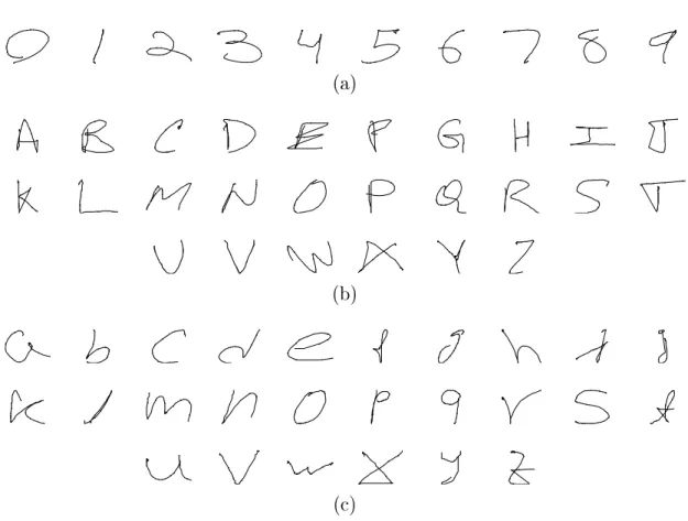
Figure 2-2: A representative example of each class of the Unipen 1a (a), Unipen 1b (b), and Unipen 1c (c) datasets.

(lowercase alphabet) datasets [27]. Figure 2-2 shows an example from each of the classes in each respective dataset. In the figure, the patterns are rendered to images, but in the dataset, they are time series consisting of 2D coordinates. The dataset consists of about 15,000 ordered sequences of pen tip coordinates and was collected by the International Unipen Foundation (iUF).

The Unipen online handwritten digit and character datasets are well established and a common source of data for time series recognition.

1URL: http://www.unipen.org/home.html

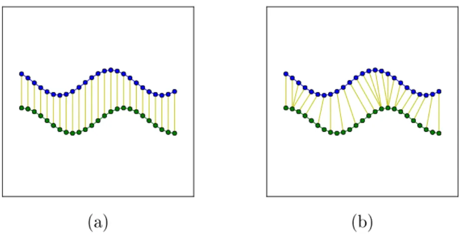
(a) (b)

Figure 2-3: A comparison to two offset time series with (a) simple linear matching of elements and (b) dynamic matching of elements. The yellow lines are pairwise matches.

2.1.2 Dynamic Time Warping (DTW)

The general idea of distance-based learning is that if a pattern has a smaller difference than one category than a second, then it typically belongs to the first category [28].

This idea is the general mechanism behind the classic pattern classification method of the nearest neighbor rule. However, determining the difference, or distance, between complex or structured patterns can be a difficult task. In this section, the use of DTW as a distance measure for time series is detailed.

Formulation of DTW

DTW is a popular algorithm to determine the difference between two discrete time

series patterns, which may vary in length and rate [29]. Shown in Fig. 2-3, DTW

tackles the problem of optimal matching of elements between two sequences. It is

possible that each step in time for one pattern does not necessarily match the same

step in time for a second pattern, thus, the general idea of dynamic matching is to

minimize the global distance by matching similar elements. In order to accomplish

this, DTW uses dynamic programming to determine the optimal matching between

elements and calculates a global distance from the summation of the local distances

between the matched elements. By dynamically matching elements, the sequences are warped in the time dimension to align similar features.

Given two discrete time series, sequence p = 𝑝

, . . . , 𝑝

, . . . , 𝑝

of length 𝐼 and sequence s = 𝑠

, . . . , 𝑠

, . . . , 𝑠

of length 𝐽 , where 𝑖 and 𝑗 are the index at each time step and 𝑝

and 𝑠

are elements at 𝑖 and 𝑗 , respectively, the global cost is the total summation of local distances between pairwise element matches. DTW estimates the minimal global cost by using the minimal warping path across the cost matrix which results in elements of each sequence being elastically matched. Figure 2-4 is a demonstration of the calculation of DTW between p and s . DTW finds the minimal total cost over an optimal warping path of a local cost matrix using dynamic programming.

DTW can be denoted as:

DTW(p, s) = ∑︁

(𝑖^′,𝑗^′)∈ℳ

𝑑 (𝑝

, 𝑠

) , (2.1)

where ℳ is the set of all matched indices (𝑖

, 𝑗

) . The matched indices 𝑖

and 𝑗

correspond to the original indices 𝑖 of p and 𝑗 of s . It should be noted that the set of matched pairs ℳ can contain repeated and skipped indices of 𝑖 and 𝑗 from the original sequences, therefore, ℳ has a nonlinear correspondence to 1, . . . , 𝑖, . . . , 𝐼 and 1, . . . , 𝑗, . . . , 𝐽 . Finally, 𝑑(·, ·) is a local distance function between elements. In DTW implementations, p is sometimes referred to as the prototype and s as a sample.

Local Distance Measure

The cost matrix is calculated using a local distance 𝑑(𝑝

, 𝑠

) between every element of sequence p and sequence s . Therefore, a suitable local distance for the domain of the particular time series must be considered.

Euclidean distance, or the L

distance, is the straight-line distance between two

points in Euclidean space. It is a natural local distance metric choice for time se-

(a) (b)

(c) (d) (e)

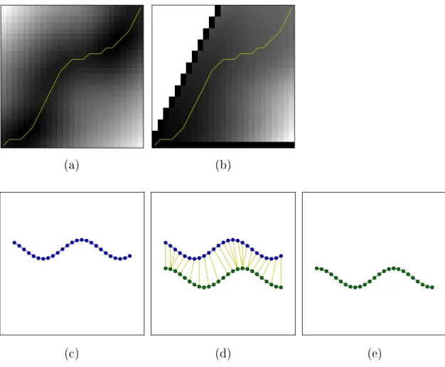
Figure 2-4: A demonstration of a DTW calculation between two time series patterns.

(a) is the cost matrix given a Euclidean cost function 𝑑(·, ·) with time series patterns (c) and (e). The shade of each square represents the distance between each pairwise element of (c) and (e). Dark pixels indicate low distance and light areas indicate high distance. The yellow line is the minimal warping path determined by dynamic programming. (b) is the cumulative sum 𝐷(·, ·) given the slope constraint in Eq. (2.3).

(d) is the optimal matching between elements in the two sequences. The yellow lines show the resulting matching between elements in each pattern.

ries with spatially related elements, such as pen tip-based handwriting and gesture tracking. DTW using Euclidean distance has been used in many works, some of which include [30, 31, 32, 33, 34, 35] and there has also been work in developing a complexity-invariant Euclidean distance [36].

While Euclidean distance is the most common, there are other local distance mea-

sures that can be used for time series analysis. DTW with Mahalanobis distance has been used for online signature verification [37], multivariate time series classifica- tion [38], and process monitoring and fault diagnosis (PM-FD) [39]. Other distance metrics used with DTW include a derivative-based DTW method [40] and Cosine distance [41, 42].

Slope Constraints

An important property of DTW is that the warping path is constrained to maintain the temporal qualities of the sequence. One of these constraints is a slope constraint.

The idea of using a slope constraint is to limit the bounds of the warping path by restricting the local route choices of the algorithm. An example symmetric slope constraint proposed by Sakoe and Chiba [43] for spoken word recognition, shown in Fig. 2-5 (a), is defined by the recurrent function:

𝐷(𝑖, 𝑗) = 𝑑(𝑝

, 𝑠

) + min

(𝑗^′,𝑖^′)∈{(𝑗,𝑖−1),(𝑗−1,𝑖−1),(𝑗−1,𝑖)}

𝐷(𝑖

, 𝑗

), (2.2) where 𝑑(𝑝

, 𝑠

) is the local cost between elements 𝑝

and 𝑠

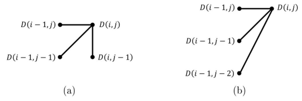
is the local cost and 𝐷(𝑖, 𝑗) is the cumulative minimum cost at the 𝑖 -th and 𝑗 -th element. The value at the cumulative sum at 𝐷(𝐼, 𝐽) is determined to be the global DTW distance between the two sequences. Figure 2-5 (b) illustrates the asymmetric slope constraint used by Itakura [44] which is defined by:

𝐷(𝑖, 𝑗) = 𝑑(𝑝

, 𝑠

) + min

𝑗^′∈{𝑗,𝑗−1,𝑗−2}

𝐷(𝑖 − 1, 𝑗

). (2.3) There are many other slope and local constraints proposed in literature [43, 45].

In addition, Kakisako et al. [35] demonstrated the use of non-Markovian local con-

straints on handwritten digit recognition. These constraints on the warping path of

the dynamic matching over the cost matrix limit reduce overfitting while allowing

flexibility to overcome local distortions.

𝐷 𝑖 − 1, 𝑗 𝐷 𝑖, 𝑗

𝐷 𝑖 − 1, 𝑗 − 1 𝐷 𝑖, 𝑗 − 1

𝐷 𝑖 − 1, 𝑗 𝐷 𝑖, 𝑗

𝐷 𝑖 − 1, 𝑗 − 1

𝐷 𝑖 − 1, 𝑗 − 2

(a) (b)

Figure 2-5: Example DTW slope constraints. Where 𝐷(𝑖, 𝑗 ) is the cumulative sum and 𝑖 and 𝑗 are the indexes of time steps given two time series p = 𝑝

, . . . , 𝑝

, . . . , 𝑝

and s = 𝑠

, . . . , 𝑠

, . . . , 𝑠

, (a) is a symmetric slope constraint and (b) is an asymmetric slope constraint.

Global Constraints

Another category of constraints are global constraints, which restrict the warping path on a global scale rather than the local scale of slope constraints. Restricting the warp- ing path on the global scale reduces the computational complexity by removing the unnecessary calculations in the regions excluded by the global constraint. Figure 2-6 illustrates three of such global constraints, the Sakoe-Chiba band [43], the Itakura parallelogram [44], and the Ratanamahatana-Keogh band [46]. In addition to reduc- ing computational complexity, the use of global constraints have shown to improve the accuracy of classification [47, 48].

The Sakoe-Chiba band, shown in Fig. 2-6 (a), creates an envelope around the warping path restricting it to a band. The intention is to prevent DTW from matching features too far apart in the sequences. The width of the band is defined by a parameter where 0% would be linear matching and 100% would be unconstrained matching. Ratanamahatana and Keogh [47] experimented with the widths of the bands and found that it depends on the dataset and testing each width would be required to find the optimal band. However, they also found that a narrower band often produces the best results.

The Itakura parallelogram, shown in Fig. 2-6 (b), is another classic global con-

(a) (b) (c)

Figure 2-6: DTW global constraints on the warping path of the cost matrix. (a) is the Sakoe-Chiba band [43]. (b) is the Itakura parallelogram [44]. (c) is the Ratanamahatana-Keogh band [46]. The white area is the permissible area of the warping path. The widths of the global constraints are set through a parameter.

straint that restricts the warping path to a parallelogram. The constraint limits the bounds of the warping path to a minimum and maximum slope. It should be noted that the asymmetric slope constraint in Eq. (2.3) also acts as a global constraint similar to a skewed Itakura parallelogram.

The Ratanamahatana-Keogh band, shown in Fig. 2-6 (c), is a more recent global constraint that trains a search for the optimal size and shape. The algorithm starts with a linear matching and expands the band based on an accuracy metric. Fur- thermore, there has been work on learning a combination of Ratanamahatana-Keogh bands [49].

DTW as a Global Distance Measure

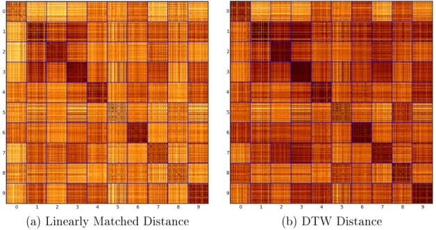
DTW has shown to be a state-of-the art distance metric for time series analysis even when compared to more modern distance metrics [34]. For example, Fig. 2-7 is the matrices of pairwise distances between 1,000 patterns from the Unipen 1a dataset.

Figure 2-7 (a) is the sum of the local Euclidean distances using a linear matching

of elements and (b) is the DTW-based distance. Darker matrix elements represent

a smaller distance, lighter matrix elements represent a larger distance, and the blue

0 1 2 3 4 5 6 7 8 9 0

1 2 3 4 5 6 7 8 9

0 600 1200 1800 2400 3000 3600 4200 4800 5400

0 1 2 3 4 5 6 7 8 9

0 1 2 3 4 5 6 7 8 9

0 500 1000 1500 2000 2500 3000 3500 4000

(a) Linearly Matched Distance (b) DTW Distance

Figure 2-7: Comparison of (a) the distance using the linear matching of elements and (b) DTW distance on the Unipen 1a (digit) dataset. The figure is the matrix of each respective distance between digit patterns and the blue lines divide the classes.

Darker is more similar and lighter is more different. 100 patterns from each class are selected at random from the dataset.

lines separate the 10 digit classes. An effective distance measure would have a larger separation between patterns of the same class and patterns of the other classes. In the figure, there is a noticeable improvement of the DTW distance matrix for class

“0,” “7,” and “8.” For those classes, there is hardly a difference between within-class and out-of-class patterns for Fig. 2-7 (a). However in the DTW distance matrix, the within-class distances are much smaller (i.e. darker) than the distances from the other classes. This demonstrates the utility of using DTW as a distance measure.

The combination of DTW as a distance measure for 𝑘 -Nearest Neighbor ( 𝑘 -NN)

has shown to be successful and very difficult to beat [50, 51, 52]. However, in recent

times, the size of available data has been increasing, and with increasingly large

datasets, exhaustive search methods such as 𝑘 -NN are not feasible for tasks that need

to be executed in reasonable amounts of time [52].

2.2 Dissimilarity Representation

Representation learning aims to learn the best representation of the data, however instead of learning from the features directly, it is possible to classify a pattern by its distance, or dissimilarity, to other patterns. While distance-based methods are common tools in pattern recognition, such as the nearest neighbor rule, it is possible to exploit vector space pattern recognition by creating feature vectors of dissimilarities.

This embedding of dissimilarities into feature vectors is referred to as Dissimilarity Space Embedding (DSE).

2.2.1 Dissimilarity Space Embedding (DSE)

DSE is a method using dissimilarity representation for vector space pattern recogni- tion. The idea is to embed sample patterns into a vector space using the dissimilarity to reference patterns (i.e. prototype patterns). The resulting vector space is an 𝑁 - dimensional vector space where 𝑁 is the number of prototype patterns. This embed- ding of dissimilarities has shown [17] to create a useful space for class discrimination.

In addition, the use of DSE allows for the foundation of vector space mathematical models and machine learning techniques to complex and structured patterns [53].

Furthermore, by creating models based on the overall distance between patterns, less emphasis is put on individual features of the patterns and more is put on how the pattern exists within the system as a whole.

This implementation of dissimilarity representation using vector spaces was intro- duced by Pekalska et al. [17] and is a currently growing field. In the original pro- posal, DSE was used for statistical data, but DSE has been further extended to the domain of graphs [54], string representations [55], and signature verification [56, 57].

In addition, other aspects of dissimilarity-based pattern recognition have been ex-

plored [58, 59, 60, 61].

𝐩

, … , 𝐩

, … , 𝐩

𝐬

𝐯

𝑑(𝐩₁, 𝒮) 𝑑(𝐩_𝑛, 𝒮)

𝑑(𝐩_𝑁, 𝒮)

𝑑(𝐩𝑛, 𝐬𝑚) 𝑑(𝐩1,𝐬𝑚) 𝑑(𝐩𝑛,𝐬𝑚)

Figure 2-8: The visualization of embedding with a sample s

in 𝒮 into an 𝑁 - dimensional vector space using the distances 𝑑(·, ·) to prototypes p

, . . . , p

, . . . , p

.

Formulation of DSE

As illustrated in Fig. 2-8, DSE uses a dissimilarity representation to create 𝑁 -dimensional dissimilarity based feature vectors to represent sample patterns. Each sample s

in 𝒮 = s

, . . . , s

, . . . , s

is represented as a vector of dissimilarities v

to each p

in 𝒫 = p

, . . . , p

, . . . , p

, or:

v

= (𝑑(p

, s

), . . . , 𝑑(p

, s

), . . . , 𝑑(p

, s

))

, (2.4) where 𝑑(·, ·) is the dissimilarity, or distance function, between patterns. Or simply, v

is the vector of each distance in 𝒫 to sample s

. Embedding dissimilarities in this way allows for the use of structural patterns to be embedded into vector space and the application of vector space recognition methods.

2.2.2 Prototype Selection for DSE

The vector space created by DSE has 𝑁 number of dimensions where 𝑁 is the num-

ber of prototype patterns. The number of prototypes used to create the space can

influence the accuracy [62]. If the number of prototypes is insufficient, then the accu-

racy of the classifier in DSE space will be low. However, if the number of prototypes

is too large, then problems arise with computational time and an increasingly high

dimensional vector space leading to the curse of dimensionality. Therefore, steps can be used toward reducing the number of prototypes or increasing the efficiency of classification.

The purpose of prototype selection is to reduce the initial set of prototypes while retaining the required information for accurate classification. In general, there are three main categories of prototype selection condensation, edition, and hybrid meth- ods [63]. Condensation methods concentrate on the samples near the decision bound- aries and remove the redundant samples away from the boundary. Edition methods take opposite approach and reduce the noise near the decision boundary for more generalized recognition. Finally, hybrid methods combine the two methods.

There are many methods of prototype selection for DSE from literature. Pekalska et al. [64] proposed using prototype clustering and other prototype selection tech- niques on DSE and Riesen and Bunke [62] extended these methods and others to graph based DSE. Pekalska et al. [65] used normal density-based classifiers in DSE to increase the efficiency of 𝑘 -NN. However, the work by Riesen et al. [62] found that there was no significant difference between the methods. The remaining of this sec- tion details the methods used for prototype selection and dimensionality reduction from literature.

Prototype Selection and Reduction Techniques for DSE

Prototype selection techniques create a subset 𝒫

of the original prototype set 𝒫 . Generally, similar patterns would create a similar dissimilarity and in turn be redun- dant for the vector space. The idea of prototype selection is to create an optimized set of prototypes which are not redundant but still carry enough information without a large degradation of accuracy. Most prototype selection techniques can be performed on the entire dataset or in a classwise fashion.

Random Selection. The most naive prototype selection method is selecting proto-

types at random. Random selection fills the subset 𝒫

with 𝑘 random patterns from

𝒫 . This process can be done per class or over the entire set of 𝒫 . Ideally, random selection creates an even density distribution of the prototypes but since they are selected in a nondirected manner, random selection is generally used as a baseline method. Random selection was used in [64] and [62] and classwise random selection was used in [64].

Center Patterns. Center pattern selection, used in [62], is a prototype selection technique of picking 𝑘 number of patterns from the center of the prototypes set. This method is not suitable for DSE because it neither reduces redundancy nor maintains useful information. However, the classwise center pattern provides a better distribu- tion of prototypes.

Border Patterns. Using border patterns takes the opposite approach as center patterns. Instead of finding the center of the prototype set, border pattern prototype selection finds the 𝑘 prototypes on the edges of the set. This method was used on graph patterns by Riesen and Bunke [62].

Similar to choosing the center patterns, using the border patterns creates a poor distribution of prototypes. Border patterns are often outlier patterns and for the purpose of creating a vector space of dissimilarities, using only the very fringe patterns cannot intuitively create a robust vector space of dissimilarities. Also similarly, this selection method could be improved using a classwise version of border patterns.

Mode Seeking. Pekalska et al. [64] proposed the use of a mode seeking method of prototype selection for dissimilarity space. Mode seeking [66] estimates the modes by using mean shift to locate the maxima of a density function. In [64], sets 𝒞 are created using mode seeking and the selected prototypes are defined as the prototypes with the minimal distances to their respective relative neighbors. The idea is to select the peaks of the 𝑘 dense clusters.

Genetic Algorithms. Genetic algorithms have a biological inspiration in that they

follow a natural selection process of evolution. A genetic algorithm solution iter-

ates through generations with small modifications to develop a best fitted solution.

Plasencia-Calana et al. [67] propose a supervised and unsupervised genetic algorithms for prototype selection of a DSE space. To select prototypes Plasencia-Calana et al. use a Minimum Spanning Tree (MST) [68] based on a unsupervised criterion and a supervised criterion using the class labels.

Condensing. Condensing [69] iterates through prototypes until all of the patterns from the training set are classified correctly. This process condenses the prototype set to only what is needed for classification. However, the number of selected proto- types is not preemptively set and depend on the complexity of the dataset. Also, the order that prototypes are selected affects the number of selected prototypes. Riesen and Bunke [62] used condensing and a modified order indiscriminate condensing al- gorithm [70] for DSE with graph patterns.

Editing. Editing [71] removes the outliers from the prototype set to reduce the noise. For this process, each pattern in the training set is classified using 𝑘 -NN and if it was misclassified, it is counted as a outlier. The prototype set is then removed of each of the outliers. Editing was used by [62] and [64] for prototype reduction for DSE.

𝑘 -Centers. Clustering is a unsupervised method of grouping similar objects and 𝑘 -Centers as a prototype selection method is the idea of using only the centers of clusters as prototypes. By only using the centers of clusters, a condensed training set is created using representative patterns that are evenly distributed with respect to dissimilarity information. This method of prototype selection was explored in [64]

for statistical data and [62] for graph data.

To implement 𝑘 -Centers for prototype selection, 𝑘 -medians clustering [72] is used.

𝑘 -Centers is a variation of the classic 𝑘 -means clustering which uses the median pat-

tern rather than the mean for clustering. The median is used so that a definite sample

is used rather than the mean sample. The 𝑘 -Centers algorithm starts with a span-

ning prototype selector with the first pattern in 𝒫

as the median and every other

pattern being the furthest away from every pattern before it. Next, it creates sets

of the nearest patterns to the initial patterns and finds the pattern in the center of each set. Then, the algorithm updates the corresponding prototype until it reaches an equilibrium with no prototypes being updated. The result is the reduced subset 𝒫

with a target size of 𝑘 that represents the centers of 𝑘 -median clusters. Also, using 𝑘 -Centers can be done classwise or over the entire prototype set.

Feature Selection Techniques for DSE

Selecting features in vector space reduces the dimensionality by using only relevant features for classification and selecting features in dissimilarity space has the same effect of prototype selection. The distinction between feature selection techniques and prototype selection techniques is that feature selection techniques are performed within the dissimilarity space.

Feature Ranking. Feature ranking is method of feature selection using a rank- ing of features based on a separability metric. In [64], Pekalska et al. use a forward feature selection [73] method with leave-one-out 1-NN for the ranking metric. The 1-NN is determined within the dissimilarity space. Eskander et al. [74] use a dis- similarity threshold optimization technique for feature selection for signature-based bio-cryptographic systems. Using an evaluation in DSE space, Eskander et al. rank the prototypes based on their discriminative power and sets a threshold to determine if the prototype should be used. Alongside reducing the number of prototypes, using a threshold also increases the accuracy by removing the confusion causing prototypes.

In addition, work has been done using other ranking metrics including Chi-square

feature ranking, information gain (InfoGain) feature ranking, and SVM recursive

feature elimination [62]. In Chi-square feature ranking, features are ranked using

multi-interval discretization [75]. The InfoGain feature ranking algorithm is based on

using mutual information to analyze the dependency of features [76]. Finally, SVM

recursive feature elimination is a feature ranking system based on ranking a SVM

classifier’s hyperplane [77].

Linear Programming. Prototypes can also be selected based on feature selection by linear programming [78]. This solution selects prototypes automatically based on separating hyperplanes in dissimilarity space. Pekalska et al. [64] used this technique to select prototypes for dissimilarity embedding.

Dimensionality Reduction Techniques for DSE

Principal Component Analysis. Jain and Spiegel [79] used Principal Component Analysis (PCA) [80] as a dimensionality reduction tool in order to reduce the num- ber of prototypes of a vector space with DSE. They demonstrated that combining PCA with Support Vector Machines (SVM) on dissimilarity representations is an effi- cient method of time series classification. PCA is a popular dimensionality reduction method that works by fitting an 𝑛 -dimensional ellipsoid to data where each axis of the ellipsoid is a principal component. It reduces the dimensionality by removing the axes with small variances. PCA was also used in [81] with 𝑘 -NN for DSE graph kernels and in [82] with generalized kernels.

𝐽 -function. Ma et al. [83] propose a dimensionality reduction of dissimilarity space using a novel method called 𝐽 -function. Linear classifiers typically perform poorly in high dimensional space but there also is a loss of data when reducing the dimensions using PCA. 𝐽 -function combines a traditional two-step procedure of using a linear classifier with PCA into a single function. Ma et al. show that allowing the classifier access to the high dimensional information while simultaneously reducing the dimensionality improves the accuracy of classification in a space created by DSE.

2.3 Deep Learning Representation

Representation learning solves the problem of representing data with learned features

over hand-crafted features. However, it is possible that the data contains complex

structures that are not solvable with pattern recognition using low-level features alone.

Deep learning attempts to solve this problem by learning high-level features built from the low-level features. Artificial Neural Networks (ANN) are the quintessential examples of deep learning representations.

2.3.1 Artificial Neural Networks (ANN)

ANNs function by stacking layers of interconnected nodes which consist of simple functions which activate based on input stimuli. The key feature of ANNs is the ability to model representations by expressing features in terms of other, lower level features. Using multiple layers of nodes, ANNs are able to map the input data to approximations of complex functions [84].

ANNs have had a long history but recently they have been the focus of the state- of-the-art research [85, 7]. There have been successes in many domains, some of which include near perfect accuracy in isolated character recognition [16], better than human performance in image classification [86], and record breaking results on established datasets [87, 88, 89].

2.3.2 Feed Forward Neural Networks

A feed forward neural network is an ANN which only maintains connections in a forward direction. The most basic feed forward neural network is a Multi-Layer Perceptron (MLP) network. Figure 2-9 (a) is an illustration of a MLP node for layer and Fig. 2-9 (b) is the network. Given an input x , feed forward neural networks approximate a function of the output x with no feedback connections. The forward flow of information and resulting approximation is called the forward propagation.

Feed forward neural networks, and more generally ANNs, train by calculating the

error to the expected result ^ y with the use of a loss function and back propagate the

error to update the weights.

∑

𝜙

…

𝑤_𝑛,5 𝑤_𝑛,4 𝑤𝑛,3

𝑤𝑛,2

𝑤_𝑛,1 𝑎𝑛

𝑥5

𝑥₄ 𝑥3

𝑥₂ 𝑥₁ 𝐰_𝑛

𝐱

𝑧𝑛

𝐚

𝑥₁ 𝑥₂ 𝑥₃ 𝑥₄ 𝑥₅

(a) (b)

Figure 2-9: Illustration of (a) an MLP node 𝑛 and (b) an MLP. x is the input elements 𝑥

, . . . , 𝑥

. w

is the weights 𝑤

, . . . , 𝑤

for each respective input. 𝑧

is the result of w

x and a is the output vector of all of the nodes.

Forward Propagation

Forward propagation, or the forward pass, is the calculation of a neural network given inputs to produce a predictive outcome. In feed forward neural networks, the layers contain nodes of simple operations. Specifically, the nodes usually contain linear classifiers, typically an inner product, with a nonlinear activation function.

The combination of stacking layers of nodes and the nonlinear activation function provides the network with the ability to learn nonlinear functions [84].

The core of the forward propagation step is the forward calculation of a node.

The activation of a node refers to if a node turns on or off and it is determined by a sum of weighted inputs. Namely, the output 𝑎

of node 𝑛 in a layer is:

𝑎

= 𝜑 (︀

w

x + 𝑏

)︀

= 𝜑 (︃

∑︁

𝑖

𝑤

𝑥

+ 𝑏

)︃

,

(2.5)

where x is a vector of the input values 𝑥

, . . . , 𝑥

, . . . , 𝑥

and w

is a vector of the respective weights 𝑤

, . . . , 𝑤

, . . . , 𝑤

to node 𝑛 and 𝜑(·) is the activation function.

The variable 𝑏

is the bias for node 𝑛 .

Activation Functions. As mentioned previously, the activation function 𝜑(·) is a nonlinear function that acts on the inner product of the weights and the inputs. The intention of the activation function is to turn on given a high enough value and turn off otherwise. In addition, activation functions typically add fuzziness near the decision boundary. Finally, the nonlinearity of the activation function allows the successive layers to combine activations to approximate nonlinear functions. Some of the most common activation functions are shown in Table 2.1.

In particular, the most common activation functions are the sigmoid, hyperbolic tangent, and rectified linear unit (ReLU) [90] activation functions. Sigmoid and hy- perbolic tangent activation functions can be seen as a soft binarization, where if the value of 𝑥 is large then the output of the activation is near 1 and when the value is very negative then the output is near 0 for sigmoid and near -1 for hyperbolic tangent. The drawback to this is that there is little difference for values of 𝑥 which are too large or too small. This phenomenon is called the vanishing gradient prob- lem and the ReLU activation function aims to prevent it by being unbounded in the positive direction. In addition, there have been attempts to improve ReLU by pre- venting ReLU from zeroing out negative values of 𝑥 with Leaky ReLU [91], Parametric ReLU (PReLU) [86], and Randomized ReLU (RReLU) [92]. However, Xu et al. [92]

found that of the rectified activations, Leaky ReLU with a small 𝛼 , thus a steep slope was particularly effective, but there is no single best function and it depends on the dataset.

Output Activation Functions. The nodes of the final layer in a network have a

specialized activation function which can be combined with a loss function for back

propagation discussed in the next section. The purpose of the specialized activation

function is to create a probability distribution of the data for classification or re-

Table 2.1: Common Activation Functions for ANNs

Name Equation Range Plot

Step 𝜑(𝑥) =

{︃ 0 for 𝑥 < 0

1 otherwise {0, 1}

−1 −0.5 0.5 1

−0.5 0.5 1

Sigmoid 𝜑(𝑥) =

(0, 1)

−4 −3 −2 −1 1 2 3 4

−0.5 0.5 1

Hyperbolic Tangent 𝜑(𝑥) = tanh 𝑥 =

− 1 (−1, 1)

−1 1

Arctangent 𝜑(𝑥) = tan

𝑥 (−

,

)

−2

−1 1 2

ReLU [90] 𝜑(𝑥) =

{︃ 0 for 𝑥 < 0

𝑥 otherwise [0, ∞)

−1 −0.5 0.5 1

−0.5 0.5 1

Leaky ReLU [91] 𝜑(𝑥) = {︃

𝛼

for 𝑥 < 0

𝑥 otherwise (−∞, ∞)

−1 −0.5 0.5 1

−0.5 0.5 1