TIME
LOCAL WELL-POSEDNESS OF
THE
COUPLED SYSTEM
OF NONLINEAR
WAVE EQUATIONS
WITH
DIFFERENT PROPAGATION SPEEDS
東北大学大学院理学研究科
津川光太郎
(Kotaro Tsugawa)
Mathematical
Institute,
Tohoku University.
1. INTRODUCTION
AND
MAIN
RESULTS
In
the
present
PaPer,
we
treat the
coupled system
of nonlinear
wave
equations
with
different
propagation speeds:
(1.1)
$(\partial_{t}^{2}-\Delta)f=F(f, \partial f,g, \partial g)$
,
$x\in \mathbb{R}^{n}$,
$t\in \mathbb{R}$,
(1.2)
$(\partial_{t}^{2}-s^{2}\Delta)g=G(f, \partial f,g, \partial g)$
,
$x\in \mathbb{R}^{n}$,
$t\in \mathbb{R}$,
(1.2)
$f(x, 0)=f_{0}(x)$
,
$\partial_{t}f(x, 0)=f_{1}(x)$
,
$x\in \mathbb{R}^{n}$,
(1.4)
$g(x, 0)=g_{0}(x)$
,
$\partial_{t}g(x, 0)=g_{1}(x)$
,
$x\in \mathbb{R}^{n}$,
where
a
$=\partial_{x_{j}}(1\leq j\leq n)$
or
$\partial_{t}$and
$s$is apropagation speed
of
(1.2)
with
$s>1$
.
The time local well-posedness
of this
system with
$s=1$
has been studied
by
many
authors. It is known
that
Strichartz’s
estimate
does
not work well to
prove the
time
local
well-posedness
of this
system
with initial data having low
regularity in
low
spatial
dimensions. However when
$s>1$
,
we
prove the time
local
well-posedness
of this
system
for
some
nonlinear terms with initial data
having
lower
regularity by taking advantage
of
the
discrepancy
of the
propagation speeds.
Let
$D=\sqrt{-\triangle}$
. We consider the following
four
cases as
the
nonlinear terms.
(Case 0)
Assume
that
$F$
and
$G$
are
any of the following functions
$FOj$
and
GOjy
$j=1,2$
,
respectively.
$F_{01}=fg$
,
$F_{02}=g^{2}$
,
$G_{01}=fg$
,
$G_{02}=f^{2}$
.
(Case 1)
Assume
that
$F$
and
$G$
are
any of the following functions
$Fij$
and
$G_{1j}$,
$j=1,2,3$ , respectively.
$F_{11}=fDg$
,
$F_{12}=gDf$
,
$F_{13}=gDg$
,
$G_{11}=fDg$
,
$G_{12}=gDf$
,
$G_{13}=fDf$
.
(Case 2)
Assume
that
$F$
and
$G$
are
any of the following
functions
$F_{2j}$and Gij,
$j=1,2$
,
respectively.
$F_{21}=D(fg)$
,
$F_{22}=D(g^{2})$
,
$G_{21}=D(fg)$
,
$G_{22}=D(f^{2})$
.
数理解析研究所講究録 1235 巻 2001 年 61-90
(Case 3)
Assume that
$F$
and
$G$
are
any of
the following
functions
$F_{3j}$and
$G_{3j}$,
$j=1,2$
,
respectively.
$F_{31}=(Df)(Dg)$
,
$F_{32}=(Dg)^{2}$
,
$G_{31}=(Df)(Dg)$
,
$G_{32}=(Df)^{2}$
.
In
Cases
1, 2and 3,
we
can
replace
the
nonlocal
operator
$D$
by the
usual derivatives
$\partial_{t}$or
$\partial_{x_{j}}$.
It does not matter
in
our
argument
below at all. This
system
has
some
physical
examples.
The time local
well-posedness
for
Klein-Gordon-Zakharov
can
essentially
be
reduced to that of
(1.1)-(1.4)
with
$F=F_{13}$
and
$G=G_{12}$
(see
[14]).
The
time
local
well-posedness
for the
coupled system
of
complex
scalar field and Maxwell
equations
can
essentially
be reduced to that of
(1.1)-(1.4)
with
$F=F_{11}+F_{12}$
and
$G=G_{13}$
(see [18]).
Our
aim is to prove the time local
well-posedness
of
(1.1)-(1.4)
with initial data
having
low regularity. Before
we
proceed
to
our
problem,
we
briefly
recall the known results. We
have the
following proposition
by
the
standard
energy
method,
the
Strichartz
estimate
and the
Sobolev
embedding.
Proposition
1.1
(known results).
Assume
that
$s>0$
. The Cauchy
problem
for
(1.1)-(1.4) is
time
locally well-posed
with initial data
$(f_{0}, f_{1})$
,
$(g_{0},g_{1})\in H^{a}\oplus H^{a-1}$
satisfying
the
assumptions
in
the following table.
Proposition
1.1 holds without the difference of the speeds. It does
not matter whether
$s=1$
or
$s\neq 1$
. Ponce and
Sideris
proved Proposition
1.1
for
$n=3$
and
Case
3in
[16].
We
can
prove the other results in
Cases
1and
2and
Case 3.
The
essence
of the
proof is
to
estimate
$D^{-1}F$
and
$D^{-1}G$
with
some
norms.
Lindblad and Sogge proved
Proposition
1.1
for
$n\geq 3$
and
Case
0in
[13].
In
Proposition 1.1,
the lower bounds
of
$a$for
$n\leq 2$
in
Cases
1and 2and
Case
3are
larger than
$(n-1)/2$
and
$(n+1)/2$
,
respectively.
One
reason
is
that the
Strichartz
estimate does not work well
in
low
spatial
dimensions. The
following
lemma is the
Strichartz
estimate. For
more
precise results,
see
[3], [5]
and
[13].
Lemma 1.1. Let
$n\geq 2,2\leq p,q\leq\infty$
satisfying
$0 \leq 2/p\leq\min\{1, (n-1)(1/2-1/q)\}$
and
$(n,p, q)\neq(3,2, \infty)$
.
If
$u$
satisfy
$(\partial_{t}^{2}-\triangle)u=0$
,
$u(x, 0)=u_{0}$
,
$\partial_{t}u(x, 0)=u_{1}$
,
then
we
have
(1.5)
$||u||_{L^{p}([0,T];\dot{B}_{q,2}^{0}(\mathrm{R}^{n}))}\leq C(||u_{0}||_{\dot{H}^{r}(\mathrm{R}^{n})}+||u_{1}||_{\dot{H}^{r-1}(\mathrm{R}^{n})})$,
where
$r=n(1/2-1/q)-1/p$
.
The
same
results hold
with
the Besov
$nom\dot{B}_{q,2}^{0}$
replaced
by
the
$L_{x}^{q}$norm, under the additional
assumption
that
$q<\infty$
.
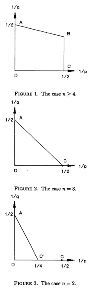
The allowed region for the
parameters
is
best pictured in the
plane
of the variables
$(1/p, 1/q)$
.
For
$n\geq 4$
,
the
allowed
region
is
aquadrangle
ABCD
with vertices
$A=$
$(0,1/2)$
,
$B=(1/2, (n-3)/2(n-1))$
,
$C=(1/2,0)$
,
$D=(0,0)$
. For
$n=3$
,
it
reduces
to
the
triangle
$ACD$
and for
$n=2$
to the smaller triangle
$AC’ D$
where
$C’=(1/4,0)$
.
See
Figures 1, 2and
3. The
limiting
case
$q=2$
occurs
only
for
$n\geq 4$
. The
boundary is
allowed
except
for the
point
$C$
for
$n=3$
. For the
$L_{x}^{q}$norm
version
of the
estimate,
the
segment
$CD$
is
excluded
by
the condition
$q<\infty$
.
In
addition,
the
$L_{x}^{q}$norm
version
of the
estimate
at the
point
$C$
for
$n=3$
is
known to be
false
([8]).
We have $r=(n-1)/2$ and
$r=3/4$
for the single
points
$C$
and
$C’$
,
respectively. These values of
$r$correspond
to the
lower
bound
of
$a$in
Cases 1and
2in Proposition
1.1.
However,
because the
segment
$CD$
is
excluded
in
the
Sobolev
version
of the
estimates,
we
need
more
derivative. Therefore,
we
have
$a>(n-1)/2$
and
$a>3/4$
in
Cases
1and 2for
$n\geq 3$
and
$n=2$
, respectively.
We note that there is agap of
1/4
derivative between the lower bound of
$a$for
Cases
1
and 2and
$(n-1)/2$
,
when
$n=2$
. We do not have the Strichartz estimate for
$n=1$
.
We
use
the
following Sobolev embedding to prove
Proposition
1.1 for
$n=1$
,
$||u||_{L_{x}}\infty\leq C||u||_{H^{r}}$
,
$r>n/2$
.
Therefore,
there
is
agap of
1/2
derivative between the lower bound of
$a$for
Cases
1and
2in Proposition
1.1 and
$(n-1)/2$
,
when
$n=1$
.
On
the other
hand,
if
we assume
$s=1$
,
Lindblad’s
counter examples [11]
and
[12] suggest that,
for
$n=3$
,
Case
0may be
time
locally ill-posed with
$a=0$
,
Cases
1and
2may be
time locally ill-posed
with
$a=1$
,
Case
3may be
time
locally ill-posed with
$a=2$
.
However,
Ozawa, Tsutaya
and
Tsutsumi
proved
the time local well-posedness
for
$n=3$
with
$F=F_{13}$
,
$G=G_{12}$
and
$s>1$
by
taking
advantage
of difference of
propagation speeds.
By combining
this result
and
the
energy
conservation law, they
showed the
time global well-posedness
of
Klein-Gordon-Zakharov
equations
for
small
initial data
(see
[14]).
By
the
same
argument, the author
[18]
showed
the time
local well
posedness
for
$n=3$
with
$F=F_{11}$
or
$F_{12}$,
$G=G_{13}$
and
$s>1$
.
By combining this result and the
energy
conservation
law the author also
showed
the time global well-posedness
of the
coupled system
of
complex
scalar
field and
Maxwell equations (see [18]).
For
more
precise
results
for
time
local
well-posedness
for
$n=3$
,
see
[15].
These results
suggest
that
the
difference of
the propagation speeds
may
be helpful to prove
the
time
local
well-posedness
with initial data
having
low
regularity.
We shall study
this
problem
for
$n=1$
and
2. The following theorem shows that the
discrepancy
of
propagation speeds
recovers
the deficiency of
1/4
and
1/2
derivative for
$n=2$
and
$n=1$
, respectively,
which reveals the
dispersive
effect hidden
in
the
Strichartz
estimate.
Theorem 1.2. Let
$s>1$
.
Then,
the Cauchy
problem
for
(1.1)-(1.4) is time locally
well-posed with
initial data
$(f_{0}, f_{1})$
,
$(g_{0},g_{1})\in H^{a}\oplus H^{a-1}$
satisfying the
assumptions in
the
following table.
$\overline{\ovalbox{\tt\small REJECT}^{-}n-2n--1}$
(Case 1)
$a>1/2$
(Case 2)
$a>1/2$
$a>0$
(Case 3)
$a>3/2$
$a>1$
(Case 1)
$a>1/2$
(Case 2)
$a>1/2$
$a>0$
(Case 3)
$a>3/2$
$a>1$
For the limiting
cases
$a=(n-1)/2$
in
Case
1and
Case
2and $a=(n+1)/2$ in
Case
3,
the following theorem holds.
Theorem
1.3. Let
$s>1$ . Then,
the Cauchy
problem
for
(1.1)-(1.4) is time locally
well-posed with initial
data
$(f_{0}, f_{1})$
,
$(g_{0}, g_{1})\in H^{a}\oplus H^{a-1}$
satisfying the
assumptions
in
$1/\mathrm{q}$
$1/\mathrm{p}$
FIGURE
1. The
case
n
$\geq 4$
.
$1/\mathrm{q}$
$1/\mathrm{p}$
$\mathrm{D}$
1/2
FIGURE
2.
The
case n
$=3$
.
$1/\mathrm{q}$
$1/\mathrm{p}$
FIGURE
3.
The
case
n
$=2$
.
the following table.
$\underline{\ovalbox{\tt\small REJECT}^{-}n-2n--1}$
(Case 1)
$F=F_{11}orF_{12}$
,
$G=G_{12}$
,
$a\geq 1/2$
(Case 2)
$F=F_{21}$
,
$G=G_{22}$
,
$a\geq 1/2$
$F=F_{21}$
,
$G=G_{21}$
,
$a\geq 0$
(Case 3)
$F=F_{31}$
,
$G=G_{32}$
,
$a\geq 32$
$F=F_{31}$
,
$G=G_{31}$
,
$a\geq 1$
(Case 1)
$F=F_{11}orF_{12}$
,
$G=G_{12}$
,
$a\geq 1/2$
(Case 2)
$F=F_{21}$
,
$G=G_{22}$
,
$a\geq 1/2$
$F=F_{21}$
,
$G=G_{21}$
,
$a\geq 0$
(Case 3)
$F=F_{31}$
,
$G=G_{32}$
,
$a\geq 3$
$2$$F=F_{31}$
,
$G=G_{31}$
,
$a\geq 1$
Moreover,
we
have
the counter
examples
of the estimates which
we
use
to prove
the
time
local
well-posedness
for other nonlinear terms for the limiting
cases
(see Proposition
3.2). However,
we
have
no
results
for
$n=2$
,
$a=1/2$
and
$F=F_{22}$
or
$F=F_{32}$
.
In
Theorems
1.2 and
1.3,
we
did not
mention the results in
Case 0for
$n\leq 2$
and
in
Case
1
for
$n=1$
,
because
there
is
another difficulty
to bring
down the lower bounds of
$a$.
For
example, in
the
case
$F=F_{21}$
,
we can
cancel the derivative
as
follows:
$D^{-1}F_{21}=D^{-1}D(fg)=fg$
.
However
in
the
case
$F=F_{11}$
,
we can
not
cancel
it.
We have
$D^{-1}F_{11}=D^{-1}(fDg)\sim D^{-1/2}(fD^{1/2}g)+D^{-1}(D^{1/2}fD^{1/2}g)$
by
the
Leibniz rule.
Therefore, it
seems
to be
difficult
to
prove the
time
local
well-posedness
for
$a<1/2$
in
Case
1. For
areason
similar to this, it
seems
to be
difficult to
prove the time local well-posedness
for
$a<0$
in
Case
0.
Indeed,
we
have
no
results
for
$a<0$
in
Case 0in
Proposition 1.1,
even
in
low spatial
dimensions.
However,
we
have
the following theorem,
which
shows
that the
discrepancy
of
propagation speeds
recover
1/4
derivative
for
some
nonlinear
terms.
Theorem
1.4.
Let
$s>1$
. Assume that
$F\neq F_{02}$
,
$G\neq G_{02}$
in
Case
0and
$F\neq F_{13}$
,
$G\neq$
$G_{13}$
in
Case 1.
Then,
the Cauchy
problem
for
(1.1)-(1.4) is time locally
$well$
-posed
with
initial data
$(f_{0}, f1)$
,
$(g_{0},g_{1})\in H^{a}\oplus H^{a-1}$
satisfying the assumptions in
the following
table.
We prove
Theorems 1.2,
1.3 and 1.4
by
the Fourier restriction
norm
method,
which
was
developed
by Bourgain [1]
and
[2]
to
study
the nonlinear
Schr\"odinger equation
and
the
$\mathrm{K}\mathrm{d}\mathrm{V}$equation,
and
it
was
improved
for the
one
dimensional
case
by
Kenig,
Ponce
and
Vega [6]
and
[7].
The related method
was
developed
by
Klainerman and
Machedon
[9]
and [10]
for
the nonlinear
wave
equations.
We
use
Fourier
restriction
norm
$X_{s,l}^{a,b}$with
$b>1/2$
to prove
Theorems 1.2 and
1.3.
We
use
not only
$X_{s,l}^{a,b}$but also slightly
different
norm
$Y_{s,l}^{a}$to prove
Theorem
1.4,
which is introduced by
Ginibre,
Tsutsumi and Velo to
study
Zakharov
system(see
[4]).
The essentially different
part
of
our
proof
from them
is only the bilinear
estimates. However,
we
state the outline
of the Fourier
restriction
norm
method
in
Section
4for
completeness
and the reader’s convenience. We mention
the bilinear
estimates
needed
for the
proof
of Theorems
1.2 and 1.4
in
Section
2and the
bilinear
estimates
needed for the
proof
of Theorems 1.2 and counter
examples in
Section
We conclude this section
by
giving
some
notations.
For
afunction
$u(t, x)$
,
we
denote
by
$\tilde{u}(\tau,\xi)$the
Fourier transform
in
both
$x$and
$t$variables
of
$u$
. For
$a$,
$b\in \mathbb{R}$,
$s>0$
and
$l=+\mathrm{o}\mathrm{r}-$
,
we
define the spaces
$X_{s,l}^{a,b}$and
$\mathrm{Y}_{s,l}^{a}$as
follows:
$X_{s,l}^{a,b}=\{u\in S’(\mathbb{R}^{3})|||u||_{X_{s,l}^{a,b}}<\infty\}$
,
$||u||_{X_{l}^{a,b}}.,=||\langle\xi\rangle^{a}P_{s,l}^{b}(\tau, \xi)\tilde{u}||_{L_{\tau,\xi}^{2}}$,
$\mathrm{Y}_{s,l}^{a}=\{u\in S’(\mathbb{R}^{3})|||u||_{Y_{s,l}^{a}}<\infty\}$
,
$||u||_{Y_{s,l}^{a}}=||\langle\xi\rangle^{a}P_{s,l}^{b}(\tau,\xi)\tilde{u}||_{L_{\xi}^{2}(L_{\tau}^{1})}$,
where
$P_{s,l}(\tau, \xi)=(1+|\tau+sl|\xi||)$
,
$\langle\xi\rangle=\sqrt{1+|\xi|^{2}}$
.
For
$T>0$,
we
denote the
cut
function
$\chi(t)$
,
$\chi \mathrm{r}(t)\in C_{0}^{\infty}$as
follows:
$\chi(t)=\{$
1for
$|t|\leq 1$
,
0for
$|t|>2$
,
$\chi\tau(t)=\chi(t/T)$
.
For
$s>0$
,
we
define
$W_{s,\pm}(t)=e^{\mp ist\omega}$
,
where
$\omega$$=\sqrt{1-\Delta}$
.
We
put
$\langle f,g\rangle=\int_{\mathrm{R}^{n+1}}f(t, x)\overline{g(t,x)}dtdx$
.
2. BILINEAR
ESTIMATES FOR
THEOREMS 1.2
AND
1.4
In this
section,
we
mention the estimates needed for the proof of Theorems 1.2 and
1.4. The following
proposition
is
the estimate which
we use
to prove
Theorem 1.2.
Proposition
2.1.
Assume
that
$a>(n-1)/2$,
$b>1/4,4a+2b>2n-1,2a+2b>n$
and
$s>1$
or $0<s<1$
. Let
$\sum_{1\leq j\leq 3}a_{j}=a$
,
$\max_{1\leq j\leq 3}a_{j}\leq a$,
$\min_{1\leq j\leq 3}a_{j}\geq-a$
.
Then,
we
have
(2.1)
$|\langle f,gh\rangle|\leq C||f||_{X_{s,j}^{a_{1},b}}||g||_{X_{1,k}^{a_{2\prime}b}}||h||_{X_{1,l}^{a_{3},b}}$,
where
$j$,
$k$and
$l$denote
either
$of+or$
-sign
and
$C$
is
a
positive
constant.
The following
proposition
is
the estimate which
we use
to prove Theorem 1.4.
Proposition
2.2.
Assume
that
$1<s$
or
$0<s<1$
.
Let
a2,
$a_{3}$,
$a_{2}+a_{3}\geq-1/2$
and
$a_{1}>n/2$
.
Then
there eist
$\epsilon>0$
and
$C>0$
such that
(2.2)
$||fg||_{X_{1.\mathrm{j}}^{-a_{1},-1/2}}\leq CT^{\epsilon}||f||_{X_{k}^{a_{2^{1/2}}}}.,’||g||_{X_{1,l}^{a_{3},1/2}}$,
(2.3)
$||fg||_{\mathrm{Y}_{1,j}^{-a_{1}}}\leq CT^{\epsilon}||f||_{X_{k}^{a_{2^{1/2}}}’}.,||g||_{X_{1,l}^{a_{3\prime}1/2}}$,
where
$j$,
$k$and
$l$denote
either
$of+or$
–sign
and
$f$
and
$g$
are
supported in
a
region
$|t|\leq T$
.
Before
we
prove Propositions 2.1 and 2.2,
we
mention preliminary lemmas.
Lemma 2.1. Let
a
$>b>0$
,
T
$>0$
and P
$=P_{s,+}$
or
$P_{s,-}$
.
Assume
that
f
is supported
in
a
region
$|t|\leq T$
.
Then,
there exists
a
positive
constant
C
such that
(2.4)
$||P^{-a}\tilde{f}||_{L_{\tau}^{2}}\leq CT^{b}||\overline{f}||_{L_{\tau}^{2}}$.
Proof.
By
H\"older’s
inequality,
we
have
(2.5)
$||P^{-a}\tilde{f}||_{L_{\tau}^{2}}=||P^{-a}\overline{\chi_{T}f}||_{L_{\tau}^{2}}\leq||P^{-a}||_{L_{\tau}^{b}}||\overline{\chi_{T}}*\tilde{f}||_{L_{\tau}^{2b/(b-2)}}$.
For
$a>b>0$
,
we
have
$||P^{-a}||_{L_{\tau}^{b}}<C$
.
By
Young’s
inequality,
we
have
(2.6)
$||\overline{\chi_{T}}*\tilde{f}||_{L_{\tau}^{2b/(b-2)}}\leq||\overline{\chi_{T}}||_{L_{\tau}^{b/(b-1)}}||\tilde{f}||_{L_{\tau}^{2}}$By
calculating directly,
we
have
(2.7)
$||\overline{\chi_{T}}||_{L_{\tau}^{b/(b-1)}}<CT^{b}$.
Collecting (2.5)-(2.7),
we
obtain (2.4).
Cl
Lemma
2.2.
Let
$0\leq c<a+b-n,$
$c \leq\min(a, b)$
and let
$l$,
$m\in \mathbb{R}^{n}$.
Then,
we
have
(2.8)
$\int_{\mathbb{R}^{n}}\langle x-l\rangle^{-a}\langle x-m,\rangle^{-b}dx\leq C\langle l-m\rangle^{-c}$,
where
$C$
is
a
positive
constant
depending only
on
$n$.
Proof.
If
$|x-l|\geq|x-m|$
then
we
have
$\langle x-l\rangle^{-a}\langle x-m\rangle^{-b}\leq\langle x-l\rangle^{-c}\langle x-m\rangle^{-a-b+c}$
and
$\langle l-m\rangle\leq\langle x-l\rangle+\langle x-m\rangle\leq 2\langle x-l\rangle$
.
Therefore,
we
have
(2.9)
$\int_{|x-l|\geq|x-m|}\langle x-l\rangle^{-a}\langle x-m\rangle^{-b}dx<C\langle l-m\rangle^{-c}\int_{\mathbb{R}^{n}}\langle x-m\rangle^{-a-b+c}dx<C\langle l-m\rangle^{-c}$
.
In
the
same
manner
we
have
(2.10)
$\int_{|x-l|\leq|x-m|}\langle x-l\rangle^{-a}\langle x-m\rangle^{-b}dx<C\langle l-m\rangle^{-c}$
.
From (2.9) and (2.10),
we
conclude
(2.8).
$\square$Lemma
2.3. Let $a>(n-1)/2$
,
$b>1/4,2a+4b>n+1$
, $2a+2b>n$
and
$s>1$
or
$0<s<1$
.
Then,
we
have
$\sup_{\tau,\xi}\frac{\langle\xi\rangle^{2a}}{P_{1,j}^{2b}(\tau,\xi)}\int_{\mathbb{R}^{n}}\int_{\mathbb{R}}\frac{1}{\langle\xi-\xi_{1}\rangle^{2a}\langle\xi_{1}\rangle^{2a}P_{1,k}^{2b}(\tau-\tau_{1},\xi-\xi_{1})P_{s,l}^{2b}(\tau_{1},\xi_{1})}d\tau_{1}d\xi_{1}<C$
where
$j,k$
and
$l$denote either
$of+or$
-sign
and
$C$
is
a
positive
constant
depending only
on
$a$,
$b$,
$s$and
$n$
.
Proof.
From Lemma
2.2
we
have
$\sup_{\tau}P_{1,j}^{-2b}(\tau, \xi)\int_{\mathbb{R}}P_{1,k}^{-2b}(\tau-\tau_{1}, \xi-\xi_{1})P_{s,l}^{-2b}(\tau_{1}, \xi_{1})d\tau_{1}$
$<C \sup_{\tau}P_{1,j}^{-2b}(\tau, \xi)(1+|\tau+k|\xi-\xi_{1}|+sl|\xi_{1}||)^{-c}<CI_{j,k,l}^{-c}$
where
$c\leq 2b,0\leq c<4b-1$
and
$I_{j,k,l}=1+|-j|\xi|+k|\xi-\xi_{1}|+ls|\xi_{1}||$
,
and
we
car
choose
$c$such
that
$c<1$
and $2a+c>n$
.
Therefore,
we
have
only
to prove
(2.11)
$\sup_{\xi}\langle\xi\rangle^{2a}\int_{\mathrm{R}^{n}}\langle\xi-\xi_{1}\rangle^{-2a}\langle\xi_{1}\rangle^{-2a}I_{j,k,l}(\xi, \xi_{1})^{-c}d\xi_{1}<C$.
We fix
$\xi$and
define
subsets
$\Omega_{1}$and
$\Omega_{2}$in
$\mathbb{R}^{n}$as
follows:
$\Omega_{1}=\{\xi_{1}\in \mathbb{R}^{n}||\xi_{1}|\geq\alpha|\xi|\}$
,
$\Omega_{2}=\{\xi_{1}\in \mathbb{R}^{n}||\xi_{1}|<\alpha|\xi|\}$
,
where
$\alpha=4/|s-1|$
.
If
$s>1$
, then
$|-j|\xi|+k|\xi-\xi_{1}|+ls|\xi_{1}||\geq s|\xi_{1}|-|\xi-\xi_{1}|-|\xi|\geq(s-1)|\xi_{1}|-2|\xi|$
.
If
$0<s<1$
, then
$|-j|\xi|+k|\xi-\xi_{1}|+ls|\xi_{1}||\geq|\xi-\xi_{1}|-s|\xi_{1}|-|\xi|\geq(1-s)|\xi_{1}|-2|\xi|$
.
Therefore, for
$\xi_{1}\in\Omega_{1}$,
we
have
(2.12)
$I_{j,k,l}>C\langle\xi_{1}\rangle$,
where
$C$
is
apositive
constant depending only
on
$s$.
Lemma
2.2 and
(2.12)
yield
(2.13)
$\langle\xi\rangle^{2a}\int_{\Omega_{1}}\langle\xi-\xi_{1}\rangle^{-2a}\langle\xi_{1}\rangle^{-2a}I_{j,k,l}^{-c}d\xi_{1}$$<C \langle\xi\rangle^{2a}\int_{\mathbb{R}^{n}}\langle\xi-\xi_{1}\rangle^{-2a}\langle\xi_{1}\rangle^{-2a-c}d\xi_{1}<C$
.
For
$\xi_{1}\in\Omega_{2}$,
we
have
(2.14)
$|-j| \xi|+k|\xi-\xi_{1}|+ls|\xi_{1}||=\frac{|s^{2}|\xi_{1}|^{2}-|\xi_{1}|^{2}+2|\xi||\xi_{1}|\cos\theta-2jls|\xi||\xi_{1}||}{|-j|\xi|-k|\xi-\xi_{1}|+ls|\xi_{1}||}$
$\geq C\frac{|\xi_{1}|}{|\xi|}|(s^{2}-1)|\xi_{1}|+2(x-jls)|\xi||$
,
where
$x=\cos\theta$
and
0is
an
angle between
4and
$\xi_{1}$.
We first consider the
case
of
$n=1$
.
We
divide
Q2
into two
parts
as
follows:
$\Omega_{21}=\{\xi_{1}\in\Omega_{2}|(s+1)|\xi_{1}|\leq|\xi|\}$
,
$\Omega_{22}=\{\xi_{1}\in\Omega_{2}|(s+1)|\xi_{1}|>|\xi|\}$
.
For
$\xi_{1}\in\Omega_{21}$,
since
(2.15)
$|(s^{2}-1)|\xi_{1}|+2(x-jls)|\xi||\geq 2|(x-jls)|\xi||-|(s^{2}-1)|\xi_{1}||$
$\geq 2|(s-1)|\xi||-|(s-1)|\xi||$
$\geq|(s-1)|\xi||\geq C|\xi_{1}|$
,
we
have
$I_{j,k,l}>C\langle\xi_{1}\rangle$
.
Therefore, in the
same manner as
(2.13),
we
obtain
(2.16)
$\langle\xi\rangle^{2a}\int_{\Omega_{21}}\langle\xi-\xi_{1}\rangle^{-2a}\langle\xi_{1}\rangle^{-2a}I_{j,k,l}^{-c}d\xi_{1}<C$.
For
$\xi_{1}\in\Omega_{22}$,
from
(2.14),
we
have
$I_{j,k,l}>C\langle|\xi_{1}|+r_{1}|\xi|\rangle$
,
where
$r_{1}=2(x-jls)/(s^{2}-1)$
.
Since
$x=1\mathrm{o}\mathrm{r}-1$
,
we
have
$|r_{1}+x|=|(.s^{2}-1)^{-1}\{2x-2jls+(s^{2}-1)x\}|$
$\leq|(s^{2}-1)^{-1}\{(s^{2}+1)x-2jls\}|>C>0$
.
Since
$n=1$
,
we
have
$|\xi-\xi_{1}|=||\xi|-x|\xi_{1}||$
.
Therefore,
from Lemma 2.2,
we
obtain
(2.17)
$\langle\xi\rangle^{2a}\int_{\Omega_{22}}\langle\xi-\xi_{1}\rangle^{-2a}\langle\xi_{1}\rangle^{-2a}I_{j,k,l}^{-c}d\xi_{1}$$\leq C\int_{\Omega_{22}}\langle|\xi|-x|\xi_{1}|\rangle^{-2a}\langle|\xi_{1}|+r_{1}|\xi|\rangle^{-c}d\xi_{1}<C$
.
From
(2. 13),(2.16)
and
(2. 17),
we
conclude
(2. 11)
for
$n=1$
.
We next consider the
case
of
$n=2$
. We divide
02
into
four
parts
as
follows:
(2.18)
$\Omega_{21}=\{\xi_{1}\in\Omega_{2}||(s^{2}-1)|\xi_{1}|+2(x-jls)|\xi||\geq\epsilon_{1}|\xi|\}$
,
(2.19)
$\Omega_{22}=\{\xi_{1}\in\Omega_{2}||(s^{2}-1)|\xi_{1}|+2(x-jls)|\xi||<\epsilon_{1}|\xi|,$
$-1+\epsilon_{1}\leq x\leq 1-\epsilon_{1}\}$
,
(2.20)
$\Omega_{23}=\{\xi_{1}\in\Omega_{2}||(s^{2}-1)|\xi_{1}|+2(x-jls)|\xi||<\epsilon_{1}|\xi|$
,
$1-\epsilon_{1}<x\leq 1\}$
,
(2.21)
$\Omega_{24}=\{\xi_{1}\in\Omega_{2}||(s^{2}-1)|\xi_{1}|+2(x-jls)|\xi||<\epsilon_{1}|\xi|,$
$-1\leq x<-1+\epsilon_{1}\}$
,
where
$\epsilon_{1}=\min\{|s-1|/2, |s-1|^{2}/4\}$
. For
$\xi_{1}\in\Omega_{21}$,
from
(2.14),
we
have
$I_{j,k,l}>C\langle\xi_{1}\rangle$
.
Therefore, in the
same manner
as
(2.13),
we
have
(2.22)
$\langle\xi\rangle^{2a}\int_{\Omega_{21}}\langle\xi-\xi_{1}\rangle^{-2a}\langle\xi_{1}\rangle^{-2a}I_{j,k,l}^{-c}d\xi_{1}<C$.
For
$\xi_{1}\in\Omega_{22}$,
since
$|\xi-\xi_{1}|^{2}=|\xi|^{2}-2|\xi||\xi_{1}|x+|\xi_{1}|^{2}$
$=x^{2}|\xi|^{2}-2|\xi||\xi_{1}|x+|\xi_{1}|^{2}+(1-x^{2})|\xi|^{2}$
$=(x|\xi|-|\xi_{1}|)^{2}+(1-x^{2})|\xi|^{2}\geq\epsilon_{1}|\xi|^{2}$
,
there
exists apositive
constant
$C$
satisfying
(2.23)
$|\xi-\xi_{1}|\geq C|\xi|$
.
From
(2.14)
and
$c<1$
,
we
have
(2.24)
$\int_{-1+\epsilon_{1}}^{1-\epsilon_{1}}I_{j,k,l}^{-c}(1-x)^{-1/2}(1+x)^{-1/2}dx\leq C\int_{-1}^{1}I_{j,k,l}^{-c}dx$
$\leq C\int_{-1}^{1}\langle|\xi_{1}|\{(s^{2}-1)\frac{|\xi_{1}|}{|\xi|}+2(x-jls)\}\rangle^{-c}dx\leq C|\xi_{1}|^{-1}\langle\xi_{1}\rangle^{1-c}$
.
Therefore,
from
(2.23)
and
(2.24),
we obtain
(2.25)
$\langle\xi\rangle^{2a}\int_{\Omega_{22}}\langle\xi-\xi_{1}\rangle^{-2a}\langle\xi_{1}\rangle^{-2a}I_{j,k,l}^{-c}d\xi_{1}$$<C \int_{0}^{\alpha|\xi|}\int_{-1+\epsilon_{1}}^{1-\epsilon_{1}}I_{j,k,l}^{-c}(1+x)^{-1/2}(1-x)^{-1/2}dx\langle\xi_{1}\rangle^{-2a}|\xi_{1}|d|\xi_{1}|<C$
$<C \int_{0}^{\alpha|\xi|}\langle\xi_{1}\rangle^{1-2a-c}d|\xi_{1}|<C$
.
For
$\xi_{1}\in\Omega_{23}$,
we
put
$r_{1}=2(x-jls)/(s^{2}-1)$
.
Then,
we
have
(2.26)
$|r_{1}| \geq\frac{2(|jls-1|-|x-1|)}{|s^{2}-1|}\geq\frac{2|s-1|-2\epsilon_{1}}{|s^{2}-1|}=\frac{1}{s+1}$
,
(2.27)
$|r_{1}+1| \geq\frac{|2x-2jls+s^{2}-1|}{|s^{2}-1|}\geq\frac{|s^{2}-2jls+1|-2|x-1|}{|s^{2}-1|}$
$\geq\frac{|s-1|^{2}}{2|s^{2}-1|}=\frac{|s-1|}{2|s+1|}$,
(2.28)
$\langle\xi-\xi_{1}\rangle\geq\langle|\xi_{1}|-|\xi|\rangle$,
(2.29)
$\langle\xi-\xi_{1}\rangle\geq C\langle|\xi_{1}|\rangle$.
From
(2.20),
we
have
$| \frac{|\xi_{1}|}{|\xi|}+r_{1}|<\frac{\epsilon_{1}}{|s^{2}-1|}$.
Therefore,
we
have
(2.30)
$\frac{|\xi_{1}|}{|\xi|}\geq|r_{1}|-\frac{\epsilon_{1}}{|s^{2}-1|}\geq\frac{2|x-jls|-\epsilon_{1}}{|s^{2}-1|}\geq\frac{2|s-1|-2|1-x|-\epsilon_{1}}{|s^{2}-1|}$
$\geq\frac{2|s-1|-3\epsilon_{1}}{|s^{2}-1|}\geq\frac{1}{2|s+1|}$
From
(2.14)
and
(2.30),
we
have
(2.31)
$I_{j,k,l}>C\langle|\xi_{1}|+r_{1}|\xi|\rangle$
Collecting
(2.26)-(2.31),
from
Lemma 2.2,
we
obtain
(2.32)
$\langle\xi\rangle^{2a}\int_{\Omega_{23}}\langle\xi-\xi_{1}\rangle^{-2a}\langle\xi_{1}\rangle^{-2a}I_{j,k,l}^{-c}d\xi_{1}$$\leq C\int_{1-\epsilon_{1}}^{1}\int_{0}^{\infty}\langle|\xi_{1}|-|\xi|\rangle^{-2a+1}\langle|\xi_{1}|+r_{1}|\xi|\rangle^{-c}d|\xi_{1}|dx<C$
.
For
$\xi_{1}\in\Omega_{24}$, in the
same
manner as
for
$\xi_{1}\in\Omega_{23}$we
have
(2.33)
$\langle\xi\rangle^{2a}\int_{\Omega_{24}}\langle\xi-\xi_{1}\rangle^{-2a}\langle\xi_{1}\rangle^{-2a}I_{j,k,l}^{-c}d\xi_{1}<C$.
$\cdot$Collecting
(2.13),(2.22),(2.25),(2.32)
and
(2.33),
we
obtain
(2.11)
for
$n=2$
.
Now,
we
prove
Propositions
2.1 and 2.2
Proof
of
Proposition
2.1. Without loss of
generality,
we can assume
$\overline{f}$,
$\overline{g}$
and
$\tilde{h}>0$
. We
first prove
(2.34)
$|\langle f,gh\rangle|\leq C||f||_{X_{1,\mathrm{j}}^{-a,b}}||g||_{X_{s,k}^{a,b}}||h||_{X_{1,l}^{a,b}}$.
By
Schwarz’s
inequality
and
Lemma 2.3,
we
have
$||\langle\xi\rangle^{a}P_{1,j}^{-b}(\tau, \xi)\{\langle\xi\rangle^{-a}P_{s,k}^{-b}(\tau, \xi)\tilde{G}*_{\tau,\xi}\langle\xi\rangle^{-a}P_{1,l}^{-b}(\tau,\xi)\tilde{H}\}||_{L_{\tau,\xi}^{2}}^{2}$
$\leq\int_{\mathbb{R}^{3}}\langle\xi\rangle^{2a}P_{1,j}^{-2b}(\tau, \xi)\{\langle\xi\rangle^{-2a}P_{s,k}^{-2b}(\tau, \xi)*_{\tau,\xi}\langle\xi\rangle^{-2a}P_{1,l}^{-2b}(\tau, \xi)\}\{\tilde{G}^{2}*_{\tau},{}_{\xi}\tilde{H}^{2}\}d\tau d\xi$
$\leq C\int_{\mathbb{R}^{3}}\tilde{G}^{2}*_{\tau},{}_{\xi}\tilde{H}^{2}d\tau d\xi\leq C||\tilde{G}^{2}||_{L_{\tau,\xi}^{1}}||\tilde{H}^{2}||_{L_{\tau,\xi}^{1}}\leq C||\tilde{G}||_{L_{\tau,\xi}^{2}}^{2}||\overline{H}||_{L_{\tau,\xi}^{2}}^{2}$
.
Substituting (4)
$aP_{s,k}^{b}(\tau, \xi)\overline{g}$for
$\tilde{G}$
and
$\langle\xi\rangle^{a}P_{1,l}^{b}(\tau, \xi)\overline{h}$for
$\tilde{H}$,
we
obtain
(2.35)
$||\langle\xi\rangle^{a}P_{1,j}^{-b}(\tau,\xi)\overline{gh}||_{L_{\tau,\xi}^{2}}\leq C||\langle\xi\rangle^{a}P_{s,k}^{b}(\tau, \xi)\overline{g}||_{L_{\tau,\xi}^{2}}||\langle\xi\rangle^{a}P_{1,l}^{b}(\tau, \xi)\overline{h}||_{L_{\tau,\xi}^{2}}$,
by the duality argument,
which
is equivalent
to
(2.34).
We
next
prove
(2.1).
We have
$|\langle f,gh\rangle|=|\langle\omega^{a_{1}-a}f,\omega^{a_{2}+a_{3}}(gh)\rangle|$
$\leq|\langle\omega^{a_{1}-a}f, (\omega^{a_{2}-a}g)(\omega^{a_{3}+a}h)\rangle|+|\langle\omega^{a_{1}-a}f, (\omega^{a_{2}+a}g)(\omega^{a_{3}-a}h)\rangle|$
,
from
(2.34),
which is
bounded
by
$C||f||_{X_{s,j}^{a_{1},b}}||g||_{X_{1,k}^{a_{2},b}}||h||_{X_{1l}^{a_{3\prime}b}}|$
.
$\square$
$\underline{P}roof$
of
Proposition
2.2. Without loss of
generality,
we
can assume
a2,
$a_{3}\leq 0,\overline{f},\overline{g}$and
$h\geq 0$
.
We
easily
see
that
(2.2)
is equivalent to
(2.36)
$|| \int_{\mathbb{R}^{n+1}}J(\tau, \xi, \tau_{1}, \xi_{1})\overline{f}(\tau-\tau_{1}, \xi-\xi_{1})\overline{g}(\tau_{1}, \xi_{1})d\tau_{1}d\xi_{1}||_{L_{\tau,\xi}^{2}}\leq CT^{\epsilon}||\tilde{f}||_{L_{\tau,\xi}^{2}}||\overline{g}||_{L_{\tau,\xi}^{2}}$,
where
$J=P_{1,j}^{-1/2}(\tau, \xi)P_{s,k}^{-1/2}(\tau-\tau_{1}, \xi-\xi_{1})P_{1,l}^{-1/2}(\tau_{1}, \xi_{1})\langle\xi\rangle^{-a_{1}}\langle\xi-\xi_{1}\rangle^{-a_{2}}\langle\xi_{1}\rangle^{-a_{3}}$,
and
(2.3)
is equivalent
to
(2.37)
$|| \int_{\mathbb{R}^{n+1}}J’(\tau, \xi, \tau_{1}, \xi_{1})\overline{f}(\tau-\tau_{1}, \xi-\xi_{1})\overline{g}(\tau_{1},\xi_{1})d\tau_{1}d\xi_{1}||_{L_{\xi}^{2}(L_{\mathcal{T}}^{1})}\leq CT^{\epsilon}||\overline{f}||_{L_{\tau,\xi}^{2}}||\tilde{g}||_{L_{\tau,\xi}^{2}}$where
$J’=P_{1,j}^{-1}(\tau, \xi)P_{s,k}^{-1/2}(\tau-\tau_{1},\xi-\xi_{1})P_{1,l}^{-1/2}(\tau_{1}, \xi_{1})\langle\xi\rangle^{-a_{1}}\langle\xi-\xi_{1}\rangle^{-a_{2}}\langle\xi_{1}\rangle^{-a_{3}}$.
we fix
$\tau$and
4and
divide the
region
of
integration into
four
parts
as
follows:
$\Omega_{1}=\{(\tau_{1}, \xi_{1})\in \mathbb{R}^{n+1}||\xi_{1}|\leq\alpha|\xi|\}$
,
$\Omega_{2}=\{(\tau_{1}, \xi_{1})\in \mathbb{R}^{n+1}||\xi_{1}|>\alpha|\xi|, P_{1,j}(\tau, \xi)\geq\max\{P_{s,k}(\tau-\tau_{1}, \xi-\xi_{1}), P_{1,l}(\tau_{1}, \xi_{1})\}\}$
,
$\Omega_{3}=\{(\tau_{1}, \xi_{1})\in \mathbb{R}^{n+1}||\xi_{1}|>\alpha|\xi|, P_{s,k}(\tau-\tau_{1},\xi-\xi_{1})\geq\max\{P_{1,j}(\tau, \xi), P_{1,l}(\tau_{1}, \xi_{1})\}\}$
,
$\Omega_{4}=\{(\tau_{1}, \xi_{1})\in \mathbb{R}^{n+1}||\xi_{1}|>\alpha|\xi|, P_{1,l}(\tau_{1}, \xi_{1})\geq\max\{P_{s,k}(\tau-\tau_{1},\xi-\xi_{1}), P_{1,j}(\tau, \xi)\}\}$
,
where
$\alpha>\max\{2/|s-1|, 2\}$
.
For
$(\tau_{1}, \xi_{1})\in\Omega_{1}$,
$\langle\xi-\xi_{1}\rangle\leq C\langle\xi\rangle$
,
$\langle\xi_{1}\rangle\leq C\langle\xi\rangle$.
Therefore
we
have
(2.38)
$J\leq C\langle\xi\rangle^{-a_{1}+1/2}P_{1_{\dot{\theta}}}^{-1/2}(\tau,\xi)P_{s,k}^{-1/2}(\tau-\tau_{1},\xi-\xi_{1})P_{1,l}^{-1/2}(\tau_{1},\xi_{1})$,
(2.39)
$J’\leq C\langle\xi\rangle^{-a_{1}+1/2}P_{1,j}^{-1}(\tau,\xi)P_{s,k}^{-1/2}(\tau-\tau_{1},\xi-\xi_{1})P_{1,l}^{-1/2}(\tau_{1},\xi_{1})$
.
From Proposition
2.1
and
(2.38),
we
have
(2.40)
$|| \int_{\Omega_{1}}J(\tau,\xi,\tau_{1}, \xi_{1})\tilde{f}(\tau-\tau_{1},\xi-\xi_{1})\tilde{g}(\tau_{1},\xi_{1})d\tau_{1}d\xi_{1}||_{L_{\tau,\xi}^{2}}$$\leq C||\langle\xi\rangle^{-a_{1}+1/2}P_{1,j}^{-1/2}\{P_{s,k}^{-1/2}\tilde{f}*_{\tau},{}_{\xi}P_{1,l}^{-1/2}\tilde{g}\}||_{L_{\tau,\xi}^{2}}$
$\leq C||P_{s,k}^{-\epsilon}\tilde{f}||_{L_{\tau,\epsilon}^{2}}||P_{1,l}^{-\epsilon}\tilde{g}||_{L_{\tau.\xi}^{2}}$
.
From
(2.39), Proposition
2.1 and
Schwarz’s
inequality,
we
have
(2.41)
$|| \int_{\Omega_{1}}J’(\tau,\xi, \tau_{1}, \xi_{1})\tilde{f}(\tau-\tau_{1},\xi-\xi_{1})\tilde{g}(\tau_{1},\xi_{1})d\tau_{1}d\xi_{1}||_{L^{2}}\epsilon^{(L_{\tau}^{1})}$$\leq C||P_{1,j}^{-1/2-\epsilon}||_{L^{\infty}(L_{\tau}^{2})}||\langle\xi\rangle^{-a_{1}+1/2}P_{1,j}^{-1/2+\epsilon}\{\epsilon P_{\epsilon,k}^{-1/2}\tilde{f}*_{\tau},{}_{\xi}P_{1,l}^{-1/2}\tilde{g}\}||_{L_{\tau}^{2}},\epsilon$
$\leq C||P_{s,k}^{-\epsilon}\tilde{f}||_{L_{\tau,\epsilon}^{2}}||P_{1,l}^{-\epsilon}\tilde{g}||_{L_{\tau.\epsilon}^{2}}$
.
For
$(\tau_{1},\xi_{1})\in\Omega_{2}$,
we
have
(2.42)
$P_{1,j}(\tau,\xi)\geq 1/3(P_{1,j}(\tau,\xi)+P_{\epsilon,k}(\tau-\tau_{1},\xi-\xi_{1})+P_{1,l}(\tau_{1},\xi_{1})$
$\geq C\langle-j|\xi|+ks|\xi-\xi_{1}|+l|\xi_{1}|\rangle$
$\geq C\langle\xi_{1}\rangle\geq C\langle\xi-\xi_{1}\rangle$
.
Therefore,
we
have
(2.43)
$J\leq C\langle\xi\rangle^{-a_{1}}P_{s,k}^{-1/2}(\tau-\tau_{1},\xi-\xi_{1})P_{1,l}^{-1/2}(\tau_{1},\xi_{1})$
,
(2.44)
$J’\leq C\langle\xi\rangle^{-a_{1}}P_{1,j}^{-1/2}(\tau,\xi)P_{s,k}^{-1/2}(\tau-\tau_{1},\xi-\xi_{1})P_{1,l}^{-1/2}(\tau_{1},\xi_{1})$
.
From
(2.43)
and Young’s inequality,
we
have
(2.45)
$|| \int_{\Omega_{2}}J(\tau,\xi, \tau_{1},\xi_{1})\tilde{f}(\tau-\tau_{1},\xi-\xi_{1})\tilde{g}(\tau_{1},\xi_{1})d\tau_{1}d\xi_{1}||_{L_{\tau,\xi}^{2}}$ $\leq C||\langle\xi\rangle^{-a_{1}}\{P_{\epsilon,k}^{-1/2}\tilde{f}*_{\tau,\xi}P_{1,l}^{-1/2}\tilde{g}\}||_{L_{\tau,\epsilon}^{2}}$ $\leq C||\langle\xi\rangle^{-a_{1}}||_{L^{2}}||P_{s,k}^{-1/2}\tilde{f}*_{\tau,\xi}P_{1,l}^{-1/2}\tilde{g}||_{L^{\infty}(L_{\tau}^{2})}\epsilon^{(L_{\tau}^{\infty})}\epsilon$ $\leq C||P_{\epsilon,k}^{-1/2}\tilde{f}||_{L^{2}}||P_{1,l}^{-1/2}\tilde{g}||_{L^{2}}\epsilon^{(L_{\tau}^{4/3})}\epsilon^{(L_{\tau}^{4/3})}$ $\leq C||P_{\epsilon,k}^{-\epsilon}\tilde{f}||_{L_{\tau.\epsilon}^{2}}||P_{1,l}^{-\epsilon}\tilde{g}||_{L_{\tau,\epsilon}^{2}}$.
72
From
(2.44)
and Young’s
inequality,
we
have
(2.46)
$|| \int_{\Omega_{2}}J’(\tau, \xi, \tau_{1},\xi_{1})\tilde{f}(\tau-\tau_{1}, \xi-\xi_{1})\tilde{g}(\tau_{1}, \xi_{1})d\tau_{1}d\xi_{1}||_{L_{\xi}^{2}(L_{\tau}^{1})}$$\leq C||\langle\xi\rangle^{-a_{1}}P_{1,j}^{-1/2}\{P_{s,k}^{-1/2}\tilde{f}*_{\tau,\xi}P_{1,l}^{-1/2}\tilde{g}\}||_{L^{2}}\epsilon^{(L_{\tau}^{1})}$
$\leq C||\langle\xi\rangle^{-a_{1}}P_{1,j}^{-1/2}||_{L_{\xi}^{2}(L_{\tau}^{\mathrm{p}})}||P_{s,k}^{-1/2}\tilde{f}*_{\tau,\xi}P_{1,l}^{-1/2}\tilde{g}||_{L_{\xi}^{\infty}(L_{\tau}^{q}\rangle}$
$\leq C||P_{s,k}^{-1/2}\tilde{f}||_{L_{\xi}^{2}(L_{\tau}^{r})}||P_{1,l}^{-1/2}\tilde{g}||_{L_{\xi}^{2}(L_{\tau}^{r})}$
$\leq C||P_{s,k}^{-\epsilon}\tilde{f}||_{L_{\tau,\xi}^{2}}||P_{1,l}^{-\epsilon}\tilde{g}||_{L_{\tau,\epsilon’}^{2}}$
where
$2<p<\infty$
,
$p^{-1}+q^{-1}=1$
and $r=2q/(q+1)>1$ .
In the
same manner as
(2.42), for
$(\tau_{1}, \xi_{1})\in\Omega_{3}$,
we
have
(2.47)
$P_{s,k}(\tau-\tau_{1}, \xi-\xi_{1})\geq C\langle\xi_{1}\rangle\geq C\langle\xi-\xi_{1}\rangle$
.
Therefore,
we
have
(2.48)
$J\leq C\langle\xi\rangle^{-a_{1}}P_{1,j}^{-1/2}(\tau, \xi)P_{1,l}^{-1/2}(\tau_{1}, \xi_{1})$,
(2.49)
$J’\leq C\langle\xi\rangle^{-a_{1}}P_{1,j}^{-1}(\tau,\xi)P_{1,l}^{-1/2}(\tau_{1},\xi_{1})$.
From
(2.48) and Young’s inequality,
we have
(2.50)
$|| \int_{\Omega_{3}}J(\tau, \xi, \tau_{1},\xi_{1})\overline{f}(\tau-\tau_{1}, \xi-\xi_{1})\overline{g}(\tau_{1}, \xi_{1})d\tau_{1}d\xi_{1}||_{L_{\tau,\xi}^{2}}$$\leq C||\langle\xi\rangle^{-a_{1}}P_{1,j}^{-1/2}\{\overline{f}*_{\tau},{}_{\xi}P_{1,l}^{-1/2}\overline{g}\}||_{L_{\tau,\xi}^{2}}$
$\leq C||\langle\xi\rangle^{-a_{1}}P_{1,j}^{-1/2}||_{L_{\xi}^{2}(L_{\tau}^{p})}||\overline{f}*_{\tau},{}_{\xi}P_{1,l}^{-1/2}\tilde{g}||_{L_{\xi}^{\infty}(L_{\tau}^{q})}$
$\leq C||\overline{f}||_{L_{\tau,\xi}^{2}}||P_{1,l}^{-1/2}\overline{g}||_{L_{\xi}^{2}(L_{\tau}^{r})}$
$\leq C||\tilde{f}||_{L_{\tau,\xi}^{2}}||P_{1,l}^{-\epsilon}\tilde{g}||_{L_{\tau,\xi}^{2}}$
,
where
$2<p<\infty$
,
$p^{-1}+q^{-1}=1/2$
and
$r=2q/(q+2)>1$
. From (2.49) and Young’s
inequality,
we
have
(2.51)
$|| \int_{\Omega_{3}}J’(\tau, \xi, \tau_{1},\xi_{1})\overline{f}(\tau-\tau_{1}, \xi-\xi_{1})\tilde{g}(\tau_{1}, \xi_{1})d\tau_{1}d\xi_{1}||_{L^{2}}\epsilon^{(L_{\tau}^{1})}$$\leq C||\langle\xi\rangle^{-a_{1}}P_{1,j}^{-1}\{\overline{f}*_{\tau},{}_{\xi}P_{1,l}^{-1/2}\tilde{g}\}||_{L_{\xi}^{2}(L_{\tau}^{1})}$
$\leq C||\langle\xi\rangle^{-a_{1}}P_{1,j}^{-1}||_{L^{2}}||\overline{f}*_{\tau},{}_{\xi}P_{1,l}^{-1/2}\tilde{g}||_{L^{\infty}(L_{\tau}^{q})}\epsilon^{(L_{\mathcal{T}}^{\mathrm{p}})}\epsilon$
$\leq C||\overline{f}||_{L_{\tau,\epsilon}^{2}}||P_{1,l}^{-1/2}\tilde{g}||_{L_{\xi}^{2}(L_{\tau}^{r})}$
$\leq C||\tilde{f}||_{L_{\tau,\epsilon}^{2}}||P_{1,l}^{-\epsilon}\overline{g}||_{L_{\tau,\epsilon’}^{2}}$
where
$1<p<2$
,
$p^{-1}+q^{-1}=1$
and $r=2q/(q+2)>1$
.
In the
same manner
as
(2.50),
we
have
(2.52)
$|| \int_{\Omega_{4}}J(\tau, \xi,\tau_{1}, \xi_{1})\overline{f}(\tau-\tau_{1}, \xi-\xi_{1})\tilde{g}(\tau_{1}, \xi_{1})d\tau_{1}d\xi_{1}||_{L_{\tau.\epsilon}^{2}}$$\leq C||P_{s,k}^{-\epsilon}\tilde{f}||_{L_{\tau,\epsilon}^{2}}||\tilde{g}||_{L_{\tau,\epsilon’}^{2}}$
In the
same manner as
(2.51),
we
have
(2.53)
$|| \int_{\Omega_{4}}J’(\tau, \xi, \tau_{1}, \xi_{1})\tilde{f}(\tau-\tau_{1}, \xi-\xi_{1})\tilde{g}(\tau_{1}, \xi_{1})d\tau_{1}d\xi_{1}||_{L_{\xi}^{2}(L_{\tau}^{1})}$$\leq C||P_{s,k}^{-\epsilon}\tilde{f}||_{L_{\tau,\xi}^{2}}||\tilde{g}||_{L_{\tau,\xi}^{2}}$
,
Prom Lemma 2.1,
(2.40),
(2.45), (2.50)
and
(2.52)
we
obtain
(2.36).
Prom Lemma
2.1,
(2.41), (2.46), (2.51)
and
(2.53)
we
obtain
(2.37).
$\square$3.
BILNEAR
ESTIMATES FOR
THEOREM
1.3
AND
COUNTER EXAMPLES
In this
section,
we
mention the estimates which
we
use
to
prove Theorem 1.3 and
counter
examples.
If
we
use
the Fourier restriction
norm
method,
we
need the
following
estimates
(3.1), (3.2)
and
(3.3)
to prove the results for the
Cases
2,3 with
$n=2$
,
for the
Case
1with
$n=2$
,
for the
Cases
2,3
with
$n=1$
,
respectively:
(3.1)
$||fg||_{\mathrm{x}_{1^{j}}^{1/2,-b’}}.,\leq C||f||_{\mathrm{x}_{2^{k}}^{1/2b}}..|||g||_{\mathrm{x}_{\mathrm{s}^{l}}^{1/2,b}’}.$,
(3.2)
$||fg||_{X_{s_{1},\mathrm{j}}^{-1/2,-b’}}\leq C||f||_{\mathrm{x}_{2^{k}}^{-1/2,b}}..||g||_{X_{s_{3},l}^{1/2,b}}$,
(3.3)
$||fg||_{X_{s_{1\prime}j}^{0,-b’}}\leq C||f||_{X_{s_{2},k}^{0,b}}||g||_{X_{s_{3},\mathrm{t}}^{0,b}}$,
for
some
$b,b’$
satisfying
$b>1/2>b’$
and
$b+b’<1$
.
Proposition
3.1. Let
$s>1,$
$b>1/2>b’$
,
$b+b’<1$
and let
$b$,
$b’$be sufficiently
close to
1/2.
i)
If
$n=2$
and
$(s_{1}, s_{2}, s_{3})=(1,1, s)$
or
$(s, 1,1)$
,
then
(3.1)
holds
for
any
$j$,
$k$,
$l=+$
$or-$
.
$\mathrm{i}\mathrm{i})$
If
$n=2$
and
$(s_{1}, s_{2}, s_{3})=(1,1, s)$
or
$(1, s, 1)$
or
$(s, 1, s)$
,
then
(3.2)
holds
for
any
$j$
,
$k$,
$l=+or-$ .
$\mathrm{i}\mathrm{i}\mathrm{i})$
If
$n=1$
and
$(s_{1}, s_{2}, s_{3})=(1,1, s)$
or
$(s, s, 1)$
,
then
(3.3)
holds
for
any
$j$,
$k$,
$l=+$
$or-$
.
Remark 3.1.
The
results for
$n=1$
follow
from Lemma
3.1
below,
which
was
proved by
Tao.
Proposition
3.2. Let
$s>1$
,
$b’\leq 1/2$
and
$(j, k, l)=(+, +, +)$
or
$($-,
$-,$
- $)$.
i)
If
$n=2$
and
$(s_{1}, s_{2}, s_{3})=(s, s, 1)$
,
then
(3.1)
fails for
any
$b\in \mathbb{R}$.
$\mathrm{i}\mathrm{i})$
If
$n=2$
and
$(s_{1}, s_{2}, s_{3})=(s, s, 1)$
or
$(1, s, s)$
or
$(s, 1,1)$
,
then
(3.2)
fails for
any
$b\in \mathbb{R}$
.
$\mathrm{i}\mathrm{i}\mathrm{i})$
If
$n=1$
and
$(s_{1}, s_{2}, s_{3})=(1, s, s)$
or
$(s, 1,1)$
,
then
(3.3)
fails for
any
$b\in \mathbb{R}$.
Remark 3.2.
Prom the result for
(3.2)
with
$n=2$
and
$(s_{1}, s_{2}, s_{3})=(s, 1, s)$
in
Proposition
3.1, (3.1)
with
$n=2$
and
$(s_{1}, s_{2}, s_{3})=(1, s, s)$
holds
for
$b’>1/2$
.
However,
for
$b’\leq 1/2$
,
we
do not know whether
(3.1)
with
$n=2$
and
$(s_{1}, s_{2}, s_{3})=(1, s, s)$
holds
or
not.
We mention
preliminary
lemmas before
we
prove
Proposition
3.1.
The
following
lemma
was
proved by
Tao
[17]
Lemma 3.1. Let
$s>1$
,
$b>1/2$
and $a=(n-1)/2$ .
Then,
we
have
(3.4)
$||fg||_{L_{x,t}^{2}}\leq C||f||_{X_{s,j}^{a,b}}||g||_{X_{1,k}^{0,b}}$,
where
$j$and
$k$denote
either
$of+or$
-sign
and
$C$
is
a
positive
constant.
Proof.
The inequality (3.4) is equivalent
to
(3.5)
$|| \int_{\mathbb{R}^{n+1}}P_{s,j}^{-b}(\tau_{1},\xi_{1})\overline{F}(\tau_{1},\xi_{1})\langle\xi_{1}\rangle^{-a}P_{1,k}^{-b}(\tau-\tau_{1}, \xi-\xi_{1})\overline{G}(\tau-\tau_{1},\xi-\xi_{1})d\tau_{1}d\xi_{1}||_{L_{\tau,\xi}^{2}}^{2}$$\leq C||\overline{F}||_{L_{\tau,\xi}^{2}}^{2}||\overline{G}||_{L_{\tau,\epsilon}^{2}}^{2}$
.
By
Schwarz’s
inequality,
the left hand side of
(3.5)
is
bounded
by
$||I^{1/2}( \int_{\mathbb{R}^{n+1}}|\tilde{F}(\tau_{1}, \xi_{1})|^{2}|\overline{G}(\tau-\tau_{1}, \xi-\xi_{1})|^{2}d\tau_{1}d\xi_{1})^{1/2}||_{L_{\tau,\epsilon}^{2}}^{2}$
$\leq\sup_{\tau,\xi}I^{2}|||\overline{F}|^{2}|\overline{G}|^{2}||_{L_{\tau,\xi}^{1}}\leq\sup_{\tau,\xi}I^{2}||\overline{F}||_{L_{\tau,\xi}^{2}}^{2}||\overline{G}||_{L_{\tau,\xi}^{2}}^{2}$
,
where
$I= \int_{\mathbb{R}^{n+1}}P_{s,j}^{-2b}(\tau_{1}, \xi_{1})\langle\xi_{1}\rangle^{-2a}P_{1,k}^{-2b}(\tau-\tau_{1}, \xi-\xi_{1})d\tau_{1}d\xi_{1}$
.
Therefore,
we
have only to
prove
$\sup_{\tau,\xi}I<C$
. From
Lemma 2.2,
we
have
$I \leq C\int_{\mathbb{R}^{n}}(1+|\tau+k|\xi-\xi_{1}|+sj|\xi_{1}||)^{-2b}\langle\xi_{1}\rangle^{-2a}d\xi_{1}$
.
Introducing polar
coordinates
$\xi$$=r\omega$
,
we
have
(3.6)
$I \leq C\int_{|\omega|=1}\int_{\mathbb{R}}(1+|j\tau+jk|\xi-r\omega|+sr|)^{-2b}drdS_{\omega}$
.
$\mathrm{B}\mathrm{e}\mathrm{c}\mathrm{a}\mathrm{u}\mathrm{s}\mathrm{e}-2b<-1$
and
$\sup_{\tau,\xi,\alpha r}\frac{d(j\tau+jk|\xi-r\omega|+sr)}{dr}\geq s-1$
,
the right hand
side of
(3.6)
is
bounded.
$\square$Lemma
3.2.
Let
$s>1$
and
$(s_{1}, s_{2}, s_{3})=(1,1, s)$
or
$(s, 1, s)$
. In the
region
$\{(\tau,\xi, \tau_{1}, \xi_{1})\in$$\mathbb{R}\cross \mathbb{R}^{2}\cross \mathbb{R}\cross \mathbb{R}^{2}||\xi-\xi_{1}|>4s|\xi|/(s-1)\}$
,
we
have
(3.7)
$\max\{P_{s_{1},j}(\tau,\xi), P_{s_{2},k}(\tau-\tau_{1}, \xi-\xi_{1}), P_{s_{3},l}(\tau_{1}, \xi_{1})\}\geq C\langle\xi-\xi_{1}\rangle$
,
(3.8)
$C’\langle\xi_{1}\rangle\geq\langle\xi-\xi_{1}\rangle\geq C’\langle\xi_{1}\rangle$,
where
$j$,
$k$and
$l$denote
either
$of+or$
-sign
and
$C$
,
$C’$
and
$C’$
are
positive
constants
depending only
on
$s$.
Remark 3.3.
In
the
region
$\{(\tau, \xi, \tau_{1}, \xi_{1})\in \mathbb{R}\cross \mathbb{R}^{2}\cross \mathbb{R}\cross \mathbb{R}^{2}||\xi|>4s|\xi-\xi_{1}|/(s-1)\}$
,
inequalities (3.7)
and
(3.8)
also hold for
$(s_{1}, s_{2}, s_{3})=(1,1, s)$
with the roles of
4and
$\xi-\xi_{1}$
exchanged
Proof.
From
$|\xi_{1}|\geq|\xi-\xi_{1}|-|\xi|\geq|\xi-\xi_{1}|-(s-1)|\xi-\xi_{1}|/4s$
,
we
have
$C’\langle\xi_{1}\rangle\geq\langle\xi-\xi_{1}\rangle$
.
From
$|\xi-\xi_{1}|\geq|\xi_{1}|-|\xi|\geq|\xi_{1}|-(s-1)|\xi-\xi_{1}|/4s$
,
we
have
$\langle\xi-\xi_{1}\rangle\geq C’\langle\xi_{1}\rangle$
.
From the triangle inequality,
we
have
$\max\{P_{\epsilon_{1},j}(\tau,\xi), P_{s_{2},k}(\tau-\tau_{1},\xi-\xi_{1}), P_{s_{3},l}(\tau_{1},\xi_{1})\}$
$\geq 1/3\{P_{\epsilon_{1},j}(\tau,\xi)+P_{\epsilon_{2\prime}k}(\tau-\tau_{1},\xi-\xi_{1})+P_{\epsilon_{3},l}(\tau_{1},\xi_{1})\}$
$\geq C\langle s_{1}j|\xi|-s_{2}k|\xi-\xi_{1}|-s_{3}l|\xi_{1}|\rangle$
.
From
$|\xi-\xi_{1}|>4s|\xi|/(s-1)$
, if
$(s_{1}, s_{2}, s_{3})=(1,1, s)$
,
then
we
have
$\sim$$|s_{1}j|\xi|-s_{2}k|\xi-\xi_{1}|-s_{3}l|\xi_{1}||\geq s|\xi_{1}|-|\xi-\xi_{1}|-|\xi|$
$\geq s|\xi-\xi_{1}|-s|\xi|-|\xi-\xi_{1}|-|\xi|$
$\geq((s-1)-(s-1)(s+1)/4s)|\xi-\xi_{1}|$
$\geq C|\xi-\xi_{1}|$
,
if
$(s_{1}, s_{2}, s_{3})=(s, 1, s)$
, then
we
have
$|s_{1}j|\xi|-s_{2}k|\xi-\xi_{1}|-s_{3}l|\xi_{1}||\geq s|\xi_{1}|-s|\xi|-|\xi-\xi_{1}|$
$\geq s|\xi-\xi_{1}|-s|\xi|-s|\xi|-|\xi-\xi_{1}|$
$\geq((s-1)-(s-1)/2)|\xi-\xi_{1}|$
$\geq C|\xi-\xi_{1}|$
.
Therefore,
we
have
(3.7).
$\square$The following
lemma is avariant
of
the
Strichartz
estimate for the acoustic
wave
equation.
For the proof
of
Lemma 3.3,
see
[2], [4]
and [6].
Lemma
3.3. Let
$s>0,2\leq q<\infty$
,
$r=4q/(q-2)$
and
$a=3/4-3/2q$
.
Then,
for
$b>1/2$
,
we
have
$||f||_{L^{r}(\mathrm{R}_{j}L^{q}(\mathrm{R}^{2}))}\leq C||f||_{X_{j}^{a,b}}.,$
’
where
$j$denotes either
$of+or$
-sign.
Now
we
prove
Proposition
3.1.
Proof of
Proposition
3.1.
i)We
first
prove
(3.1)
with
$n=2$
and
$(s_{1}, s_{2}, s_{3})=(s, 1,1)$
.
The inequality
(3.1)
is equivalent to
(3.9)
$||P_{\epsilon,j}^{-b’}( \tau,\xi)\langle\xi\rangle^{1/2}\int_{\mathrm{R}^{2+1}}P_{1,k}^{-b}(\tau-\tau_{1},\xi-\xi_{1})\langle\xi-\xi_{1}\rangle^{-1/2}\tilde{F}(\tau-\tau_{1},\xi-\xi_{1})$$\cross$ $P_{1,l}^{-b}(\tau_{1},\xi_{1})\langle\xi_{1}\rangle^{-1/2}\tilde{G}(\tau_{1},\xi_{1})d\tau_{1}d\xi_{1}||_{L_{\tau,\xi}^{2}}^{2}$
$\leq C||\tilde{F}||_{L_{\tau,\epsilon}^{2}}^{2}||\tilde{G}||_{L_{\tau,\xi}^{2}}^{2}$
.
Without
loss of
generality,
we can
assume
$\tilde{F}\geq 0$and
$\tilde{G}\geq 0$.
We divide
$(\tau,\xi)\in \mathbb{R}^{3}$into
two parts
as
follows:
$A_{1}=\{(\tau, \xi)||\tau+sj|\xi||>\epsilon|\xi|\}$
,
$A_{2}=\{(\tau, \xi)||\tau+sj|\xi||<\epsilon|\xi|\}$
,
where
$\epsilon>0$
and
$\epsilon$is sufficiently small
to
be
determined later.
$\mathrm{a})\mathrm{F}\mathrm{o}\mathrm{r}(\tau, ()$ $\in A_{1}$
,
we
have
$P_{s,j}^{-b’}(\tau, \xi)\langle\xi\rangle^{1/2}\leq C\langle\xi\rangle^{1/2-b’}\leq C\langle\xi-\xi_{1}\rangle^{1/2-b’}+C\langle\xi_{1}\rangle^{1/2-b’}$
Therefore,
we
have
(3.10)
$||P_{s,j}^{-b’}( \tau,\xi)\langle\xi\rangle^{1/2}\int_{\mathbb{R}^{2+1}}P_{1,k}^{-b}(\tau-\tau_{1}, \xi-\xi_{1})\langle\xi-\xi_{1}\rangle^{-1/2}\tilde{F}(\tau-\tau_{1}, \xi-\xi_{1})$$\cross P_{1,l}^{-b}(\tau_{1}, \xi_{1})\langle\xi_{1}\rangle^{-1/2}\tilde{G}(\tau_{1},\xi_{1})d\tau_{1}d\xi_{1}||_{L^{2}(A_{1})}^{2}$
$\leq C||P_{1,k}^{-b}\langle\xi\rangle^{-b’}\overline{F}*_{\tau},{}_{\xi}P_{1,l}^{-b}\langle\xi\rangle^{-1/2}\overline{G}||_{L_{\tau,\epsilon}^{2}}^{2}+C||P_{1,k}^{-b}\langle\xi\rangle^{-1/2}\tilde{F}*_{\tau},{}_{\xi}P_{1,l}^{-b}\langle\xi\rangle^{-b’}\tilde{G}||_{L_{\tau,\xi}^{2}}^{2}$
From
H\"older’s
inequality,
Plancherel’s theorem and Lemma 3.3,
we
have
(3.11)
$||P_{1,k}^{-b}\langle\xi\rangle^{-b’}\overline{F}*_{\tau},{}_{\xi}P_{s,l}^{-b}\langle\xi\rangle^{-1/2}\overline{G}||_{L_{\tau,\epsilon}^{2}}^{2}$$\leq C||\mathcal{F}_{\tau,\xi}^{-1}(P_{1,k}^{-b}\langle\xi\rangle^{-b’}\overline{F})||_{L_{t,x}^{3}}^{2}||\mathcal{F}_{\tau,\xi}^{-1}(P_{s,l}^{-b}\langle\xi\rangle^{-1/2}\overline{G})||_{L_{t,x}^{6}}^{2}$
$\leq C||\overline{F}||_{L_{\tau,\xi}^{2}}^{2}||\overline{G}||_{L_{\tau,\xi}^{2}}^{2}$
.
In the
same
manner we
have
(3.12)
$||P_{1,k}^{-b}\langle\xi\rangle^{-1/2}\overline{F}*_{\tau},{}_{\xi}P_{s,l}^{-b}\langle\xi\rangle^{-b’}\overline{G}||_{L_{\tau,\epsilon}^{2}}^{2}\leq C||\overline{F}||_{L_{\tau,\xi}^{2}}^{2}||\overline{G}||_{L_{\tau,\xi}^{2}}^{2}$.
Collecting (3.10)-(3.12),
we
have
(3.13)
$||P_{s,j}^{-b’}( \tau, \xi)\langle\xi\rangle^{1/2}\int_{\mathbb{R}^{2+1}}P_{1,k}^{-b}(\tau-\tau_{1}, \xi-\xi_{1})\langle\xi-\xi_{1}\rangle^{-1/2}\overline{F}(\tau-\tau_{1}, \xi-\xi_{1})$$\cross P_{1,l}^{-b}(\tau_{1}, \xi_{1})\langle\xi_{1}\rangle^{-1/2}\overline{G}(\tau_{1}, \xi_{1})d\tau_{1}d\xi_{1}||_{L^{2}(A_{1})}^{2}$
$\leq C||\overline{F}||_{L_{\tau,\xi}^{2}}^{2}[|\overline{G}||_{L_{\tau,\xi}^{2}}^{2}$
.
$\mathrm{b})\mathrm{F}\mathrm{o}\mathrm{r}(\tau,\xi)\in A_{2}$
,
we
devide
$(\tau_{1}, \xi_{1})\in \mathbb{R}^{3}$into three
parts
as
follows:
$\Omega_{1}=\{(\tau_{1},\xi_{1})||\tau-\tau_{1}+k|\xi-\xi_{1}||>\epsilon|\xi|\}$
,
$\Omega_{2}=\{(\tau_{1},\xi_{1})||\tau_{1}+l|\xi_{1}||>\epsilon|\xi|\}$
,
$\Omega_{3}=\{(\tau_{1},\xi_{1})|\max\{|\tau-\tau_{1}+k|\xi-\xi_{1}||, |\tau_{1}+l|\xi_{1}||\}<\epsilon|\xi|\}$
.
For
$(\tau_{1},\xi_{1})\in\Omega_{1}$,
we
have
$P_{1,k}^{-b}(\tau-\tau_{1}, \xi-\xi_{1})\langle\xi\rangle^{1/2}\leq C$
.
Therefore,
we
have
(3.14)
$||P_{s,j}^{-b’}( \tau, \xi)\langle\xi\rangle^{1/2}\int_{\Omega_{1}}P_{1,k}^{-b}(\tau-\tau_{1}, \xi-\xi_{1})\langle\xi-\xi_{1}\rangle^{-1/2}\overline{F}(\tau-\tau_{1}, \xi-\xi_{1})$$\cross P_{1,l}^{-b}(\tau_{1},\xi_{1})\langle\xi_{1}\rangle^{-1/2}\tilde{G}(\tau_{1},\xi_{1})d\tau_{1}d\xi_{1}||_{L^{2}(A_{2})}^{2}$
$\leq C||\langle\xi-\xi_{1}\rangle^{-1/2}\overline{F}*_{\tau},{}_{\xi}P_{s,l}^{-b}\langle\xi\rangle^{-1/2}\tilde{G}||_{L_{\tau,\xi}^{2}}^{2}$
.
Prom
H\"older’s
inequality,
Plancherel’s
theorem and
the Sobolev
embedding,
we
have
(3.15)
$||\langle\xi-\xi_{1}\rangle^{-1/2}\overline{F}*_{\tau},{}_{\xi}P_{s,l}^{-b}\langle\xi\rangle^{-1/2}\overline{G}||_{L_{\tau,\epsilon}^{2}}^{2}$$\leq C||\omega^{-1/2}F||_{L_{t}^{2}(L_{x}^{4})}^{2}||\mathcal{F}_{\tau,\xi}^{-1}(P_{s,l}^{-b}\langle\xi\rangle^{-1/2}\tilde{G})||_{L_{t}^{\infty}(L_{x}^{4})}^{2}$
$\leq C||\tilde{F}||_{L_{\tau,\xi}^{2}}^{2}||\tilde{G}||_{L_{\tau,\epsilon}^{2}}^{2}$
.
Prom
(3.14)
and
(3.15),
we
have
(3.16)
$||P_{s,j}^{-b’}( \tau, \xi)\langle\xi\rangle^{1/2}\int_{\Omega_{1}}P_{1,k}^{-b}(\tau-\tau_{1},\xi-\xi_{1})\langle\xi-\xi_{1}\rangle^{-1/2}\tilde{F}(\tau-\tau_{1}, \xi-\xi_{1})$$\cross P_{1,l}^{-b}(\tau_{1},\xi_{1})\langle\xi_{1}\rangle^{-1/2}\tilde{G}(\tau_{1},\xi_{1})d\tau_{1}d\xi_{1}||_{L^{2}(A_{2})}^{2}$
$\leq C||\tilde{F}||_{L_{\tau,\xi}^{2}}^{2}||\tilde{G}||_{L_{\tau,\epsilon}^{2}}^{2}$
.
In
the
same
manner we
have
(3.17)
$||P_{s,j}^{-b’}( \tau,\xi)\langle\xi\rangle^{1/2}\int_{\Omega_{2}}P_{1,k}^{-b}(\tau-\tau_{1},\xi-\xi_{1})\langle\xi-\xi_{1}\rangle^{-1/2}\tilde{F}(\tau-\tau_{1}, \xi-\xi_{1})$$\cross P_{1,l}^{-b}(\tau_{1},\xi_{1})\langle\xi_{1}\rangle^{-1/2}\tilde{G}(\tau_{1}, \xi_{1})d\tau_{1}d\xi_{1}||_{L^{2}(A_{2})}^{2}$
$\leq C||\tilde{F}||_{L_{\tau.\epsilon}^{2}}^{2}||\tilde{G}||_{L_{\tau,\xi}^{2}}^{2}$
.
We
put
$I( \tau,\xi)=P_{\epsilon_{\dot{\theta}}}^{-2b’}(\tau,\xi)\langle\xi\rangle\int_{\Omega_{3}}P_{1,k}^{-2b}(\tau-\tau_{1},\xi-\xi_{1})\langle\xi-\xi_{1}\rangle^{-1}P_{1,l}^{-2b}(\tau_{1},\xi_{1})\langle\xi_{1}\rangle^{-1}d\tau_{1}d\xi_{1}$
.
If
we
have
(3.18)
$\sup I(r, \xi)<C$
,
$(\tau,\xi)\in A_{2}$
then,
by
Schwarz’s
inequality,
we
have
(3.19)
$||P_{\epsilon,j}^{-b’}( \tau, \xi)\langle\xi\rangle^{1/2}\int_{\Omega_{3}}P_{1,k}^{-b}(\tau-\tau_{1},\xi-\xi_{1})\langle\xi-\xi_{1}\rangle^{-1/2}\tilde{F}(\tau-\tau_{1}, \xi-\xi_{1})$$\cross P_{1,l}^{-b}(\tau_{1},\xi_{1})\langle\xi_{1}\rangle^{-1/2}\tilde{G}(\tau_{1},\xi_{1})d\tau_{1}d\xi_{1}||_{L^{2}(A_{2})}^{2}$
$\leq C||I^{1/2}(\int_{\mathbb{R}^{3}}|\tilde{F}(\tau_{1},\xi_{1})|^{2}|\tilde{G}(\tau-\tau_{1}, \xi-\xi_{1})|^{2}d\tau_{1}d\xi_{1})^{1/2}||_{L_{\tau,\xi}^{2}}^{2}$
$\leq C|||\tilde{F}|^{2}*_{\tau,\xi}|\tilde{G}|^{2}||_{L_{\tau,\epsilon}^{1}}$
$\leq C||\tilde{F}||_{L_{\tau,\epsilon}^{2}}^{2}||\tilde{G}||_{L_{\tau,\xi}^{2}}^{2}$