Realistic models of computability
on
the
real numbers
Vasco Brattka
Theoretische Informatik I, $\mathrm{F}\mathrm{e}\mathrm{r}\mathrm{n}\mathrm{U}\mathrm{n}\mathrm{i}\mathrm{v}\mathrm{e}\mathrm{r}\mathrm{s}\mathrm{i}\mathrm{t}\dot{\mathrm{a}}\mathrm{t}$Hagen, D-58084 Hagen, Germany
$\mathrm{e}$-mail: [email protected]
April 26,
2000
Abstract
In this paper we discuss the role of the model of computability in the cycle
of real number programming. We argue that problems occurring in practice, like
instability or degeneracy problems, are caused by the real number model. As a
morerealisticapproach we propose the point ofview ofcomputableanalysis andwe
present a feasible real number model which is compatible to this approach. Finally,
we briefly discuss a general theory of continuous data structures which is based on
computable analysis.
Keywords: real number model, computable analysis, continuous data structures.
1
Introduction
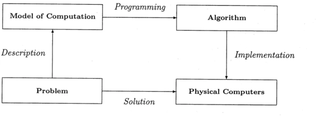
We will start to discuss the role of the model of real number computation in the cycle of real number programming. Typically, this cycle can be characterized by the following three steps (cf. Figure 1):
(1) Description: in a first step the problem under consideration is described in terms which are offered by some given model of computation on the real numbers.
(2) Programming: in a second step themodel of computation is used to develop some
algorithm which solves the problem. Thus, “programming” here means “developing algorithms”
(3) Implementation: last not least, the algorithm is implemented in some concrete
programming language on a physical computer.
It is easy to realize that this cycle of real number programming sensitively relies on
the chosen model of computability on the real numbers. This model already determines
the description of the problem,
as
wellas
the construction of the algorithm. Moreover, it depends onthe model ofcomputability whether acorrectimplementationof the algorithmon physical computers will be possible or not.
It is the real number model which is used as the standard model of computability on
Figure 1: The cycle of real number programming
based on the idea that real numbers are entities and formally it is introduced via register machines or so-called real random
access
machines which are equipped with real number registers and whichcanperform arithmeticoperationsas
wellas comparisons and equalitytests
on
real numbers precisely.Therealnumber modelisthe standardmodel incomputationalgeometry (cf. Preparata
and Shamos [PS85]$)$; it has been used by Blum, Shub and Smale
[BSS89] to introduce a theory of computational complexity and by Traub, Wasilkowski and Woz’niakowsky
[TWW88] to describe the complexity of algorithms in numerical analysis.
From acertainpoint of view the real number model is the mathematical
formalization
of the semantics which is offered by typical imperative programming languages on the real numbers. Languages like JAVA, $\mathrm{C}$,
PASCAL
and FORTRANoffer a data type “real” together with arithmetic operations and comparisons. But unfortunately, this semantics
cannot be realized precisely on physical computers. This is not just a precision problem
of floating point arithmetic but it is a general limitation of physical computers.
Heuristically, the problems of the real number model are well-known to practitioners,
$\mathrm{e}.\mathrm{g}$. numerical analysts know that comparisons with zero
can
be problematic and haveto be avoided. Special terminologies have been invented to describe the problems: the
problem under consideration canbe called ill-conditioned, or aspecific input canbe called
degenerated, or the algorithm can be called instable.
Rom the point of view ofcomputable analysis the cardinal problem is that real
num-bersare infiniteobjects and infinitetimewe canonlyhandle finiteportionsofinformation.
Consequently, discontinuous problems cannot be solved by physical machines. Especially,
the precise comparisons and equality tests of the real number model cannot be performed by physical computers.
The importance of the discontinuityproblem depends on the specific area of
applica-tion. For instance, in numerical analysis most of the algorithms treat continuous problems like numerical integration; discontinuous problemslike numericaldifferentiation have been realized as unsolvable in the general case. Even if an algorithm uses
some
discontinuoustest (like the Heron algorithm) this causes no problems in practice, since the
correspond-ing problem is continuous (likethe square root function). The situation in computational
discon-tinuous (e.g. test whether a point belongs to some convex hull) and thus they cannot be
solved without the discontinuous basic operations of the real number model (cf. Hertling
and Weihrauch [HW94] and Burnikel, Mehlhorn, and Schirra [BMS94]$)$. In the worst
case
this can lead to algorithms which map typical inputs to completely incorrect outputs. This phenomenon can also be illustrated by the function
$f$ $:\subseteq \mathbb{R}arrow \mathbb{R},$ $(x, y)-\rangle\{$
1 if$x\in \mathbb{Q}$
$0$ if$x\not\in \mathbb{Q},$$x^{2}\in \mathbb{Q}$
)
undefined in all other cases, which
can
be computed according to the real number modelbut which canneither be approximately computed inarealistic
sense
nor be implemented correctly using floating point arithmetic (cf. Weihrauch $[\mathrm{W}\mathrm{e}\mathrm{i}98|$).This highly unsatisfactory situation could be resolved by a Copernican turn: instead
ofdevelopingthebest possible algorithms according to the real numbermodel,
one
shouldsearch for the best possible model according to the abilities and limitations of physical computers. As
soon as
such a model has been discovered, computer scientists should feel free to replace the semantics of imperative programming languages by a semantics which perfectly fits together with the new model.Computable analysis is the right tool to figure out such a realistic model because it is based on Turing machines. Following Church’s thesis, we can
assume
that Turing machines describe the possibilities of handling finite information by physical machines in the most realistic way according to our current knowledge.We close the introduction with a short survey on the organization of the paper: in
the following Section 2 we will shortly discuss the model of computability which is used in computable analysis. In Section 3
we
present the feasible real randomaccess
machinemodel, which has been introduced in a joint project with Peter Hertling [BH98] and
which is a realistic modification of the real number model with respect
to
computability and complexity. Finally, in Section 4 we briefly discuss a general theory of continuous data structures and we sketch how the ideas that have been applied to the real numberscan
be transferred to other objects like compact sets and continuous functions.2
Computable analysis
Inthis sectionwewould like to presentsome basic definitions and results from computable
analysis which show how a realistic Turing machine based model of computability on the
real numbers can be defined. The origins of computable analysis go back to Turing’s
paper [Tur36] in which he presented his famous machine model. It is not very
well-known that
one
of his purposeswas
to introduce a formal definition for the notion of acomputable real number. The corresponding notionof acomputable real number function has systematically been studied by Grzegorczyk [Grz57] and Lacombe [Lac55] in the fiftieth. Later on, the theory of computable analysis has been developed by Hauck [Hau73],
Pour-El and Richards [PER89], Ko [Ko91] and Kreitz and Weihrauch [KW84] and many
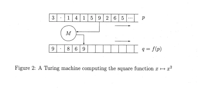
Figure 2: A Turing machine computing the square function $x-\rangle$ $x^{2}$
of computable analysis can be described in the following way: fix
some
representationof the real numbers by infinite sequences and call a real number function computable, if there exists a Turing machine that transfers each sequence which represents
some
inputinto a sequence which represents the corresponding output of the function. Figure 2
illustrates the situation for the square function with input $\pi$ in decimal representation.
More formally,
we
will first fix the notion ofa
representation.Definition 2.1 (Representation) Arepresentationofthe real numbers$\mathbb{R}$is asurjective
function $\delta:\subseteq\Sigma^{\omega}arrow \mathbb{R}$.
Here $\Sigma^{\omega}$ denotes the set ofinfinite sequencesoverthe alphabet $\Sigma$ the inclusion symbol $”\subseteq$” indicates a potentially partial functions. An example of a representation
is the ordinary decimal representation. Now it is straightforward to define the notion of a
computable real number function.
Definition 2.2 (Computable real number function) A function $f:\subseteq \mathbb{R}arrow \mathbb{R}$ is
called computable with respect to some representation $\delta:\subseteq\Sigma^{\omega}arrow \mathbb{R}$, if there exists
some
Turing machine $M$ (with one-way output tape) which computesinfinitely long and whichin the long run transforms each sequence $p\in\Sigma^{\omega}$ which represents
some
$x:=\delta(p)\in \mathbb{R}$into some sequence $q\in\Sigma^{\omega}$ which represents $f(x)$, i.e. $f(x\grave{)}=\delta(q)$.
It is straightforward how to extend this definition to multi-dimensional functions
$f:\subseteq \mathbb{R}^{n}arrow \mathbb{R}$. It is easy to observe that this definition of a computable real number
function sensitively relies on the chosen representation of the real numbers. Turing, who
chosethe ordinary decimal representation of the real number in his first attempt, realized in a correction of his famous paper [Tur37] that the decimal representation has
some
se-rious disadvantages and other representations are preferable. Especially, he realized the following:
Proposition 2.3 (Decimal representation) Multiplication by 3, $i.e$. the real
function
$f$ : $\mathbb{R}arrow \mathbb{R},$$x->3x$ is not computable with respect to the decimal representation.
The proof by contradiction is quite easy: each machine which would compute
either to $q=$ 0.9999... or to $q’=$
1.0000....
Especially, the machine has to write 0.9 or1.0 on the output tape after some finite time, but no finite prefix of the input sequence$p$
suffices to decide whether the correct output sequence has to start with 0.9 or with 1.0.
Consequently, such a machine cannot exist.
As a consequence of this phenomenon Turing did not abandon his machine model
for computations with real numbers but he replaced the decimal representation by some
other representation. One possible choice of some reasonable representation is the
so-called “signed-digit $\mathrm{r}\mathrm{e}\mathrm{p}\mathrm{r}\mathrm{e}\mathrm{s}\mathrm{e}\mathrm{n}\mathrm{t}\mathrm{a}\mathrm{t}\mathrm{i}\mathrm{o}\mathrm{n}^{)}$’ which is defined like the decimal representation but
which also allows negative digits. Fromnow on we will assumethat $\delta$ is thebinary
signed-digit representation of the real numbers which operates with base 2 and signed-digits $-1,0,1$ .
Computability of real number functions will be understood w.r.t. this representation. Most concrete continuous functions which are used in analysis are computable in this
sense.
Proposition 2.4 (Computable real functions) The real arithmetic $operations+,$ -,
$.,$ $\div:\subseteq \mathbb{R}^{2}arrow \mathbb{R}$ and the
functions
$\mathrm{s}\mathrm{i}\mathrm{n},$
$\mathrm{c}\mathrm{o}\mathrm{s},$ $\exp$ :
$\mathbb{R}arrow \mathbb{R}$ are computable real number
functions.
The proof for this and the following results in this section can be found in [WeiOO].
One of the main observations of computable analysis is that all computable real number functions are continuous.
Theorem 2.5 (Continuity of computable functions) All computable real
functions
$f$ $:\subseteq \mathbb{R}^{n}arrow \mathbb{R}$ are continuous.
Since each finite prefix of the output has to be computed from some finite prefix of
the input, each finite prefix of the output has at least to depend on some finite prefix of
the input. But this dependency is nothing but continuity. As a direct consequence one
obtains that the equality test on the real numbers is not decidable.
Proposition 2.6 (Undecidability of the equality) The equality test onthe real
num-bers is not decidable, $i.e$. the
function
$e$ : $\mathbb{R}^{2}arrow \mathbb{R},$ $(x, y)\mapsto\{$
$0$
if
$x=y$1 else is not computable.
Now one could ask whether the undecidability of the equality is just a bad property
of the signed-digit representation (in the
same sense
as the non-computability of the multiplication by 3 is just a bad property of the decimal representation). Unfortunately, there is an easy cardinality argument which shows that equality is undecidable with respect to all representations of the real numbers [WeiOO]. In other words: there is noReal number model Computable analysis arbitrary constants only computable constants
arithmetic operations are computable arithmetic operation are computable
precise tests $=,$ $<$ only finite precision tests
$\mathrm{s}\mathrm{i}\mathrm{n},$
$\mathrm{c}\mathrm{o}\mathrm{s},$ $\exp$ are not computable $\mathrm{s}\mathrm{i}\mathrm{n},$
$\mathrm{c}\mathrm{o}\mathrm{s},$ $\exp$ are computable
Table 1: Models of computability on the real numbers
The following table summarizes some joint properties and some differences between the real number model and the model of computability as it is used in computable analysis.
The property stated in the first line of the table is due to the fact that in the formal-ization of the real number model of Blum, Shub and Smale [BSS89] arbitrary constants
are allowed. This enables BSS machines to decide arbitrary discrete problems (the char-acteristic function can simply be stored in a constant). Thus, if one insists on arbitrary constants then the model is not only unrealistic for topological
reasons
but also forrecur-sion theoretic
reasons.
Moreover, the basic real number model is not only unrealistic but also incomplete, since many important functions (like the trigonometric functions) arenot computable in this model because it does not offer any limit construction. Finally, also the class of recursive sets which have been defined with the help of the real number model is not very reasonable, since easy sets like the graph or the closed epigraph of the
exponential functions are not recursive in this sense $[\mathrm{B}\mathrm{r}\mathrm{a}99\mathrm{a}]$.
3
Feasible real
random
access
machines
In the previous section we have seen how a realistic Turing machine based model of computability on the real numbers can be defined. One problem related to this model is that it will be difficult to convince practitioners in computational geometry or numerical analysis to describe their algorithms in terms of Turing machines. In this section we
would like to introduce the so-called feasible real random access machine model (feasible RAM) which overcomes this problem since it characterizes the Turing machine approach
ofcomputable analysis intermsas closeas possible to the real number model. The feasible
real random
access
machinemodelas
wellas
all presented resultsare due to ajoint project with Peter Hertling [BH98]. The feasible real RAM can be characterized by the following features:$\bullet$ rational constants,
$\bullet$ usual arithmetic operations on $\mathrm{N}$ and $\mathbb{R}$,
$\bullet$ ordinary tests $<,$$=\mathrm{o}\mathrm{n}\mathrm{N}$,
$\bullet$ approximative semantics,
$\bullet$ logarithmic time complexity
measure.
We will not formalize the definition of our feasible real RAMs but we will describe it
intuitively. Roughly speaking, a feasible real RAM is a register machine with two types
of registers: natural number registers $n_{i}$ and real number registers $r_{j}$. A finite number of these registers can be used
as
input and output registers. The program of a feasible realRAM is controlled by
some
finite flowchart. A precise list of all basic operations whichare allowed in flowcharts ofthe feasible real
RAM
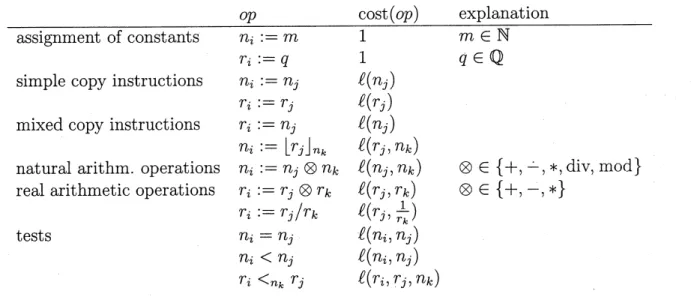
together with there logarithmic costsis given in the following table. The logarithmic cost $\ell(x)$ denotes roughly speaking the
length of the binary representation of the integer part of $x$. More precisely, for $x\in \mathrm{N}$
or $x\in \mathbb{R}$ we
use
$\ell(x)=1+\lfloor\log(\max\{|x|, 1\})\rfloor$. Here $\log$ denotes the binary logarithm: $\log(x):=\log_{2}(x)$.$op$ cost$(op)$ explanation
assignment of constants $n_{i}:=m$ 1 $m\in \mathrm{N}$
$r_{i}:=q$ 1 $q\in \mathbb{Q}$
simple copy instructions $n_{i}:=n_{j}$ $l(n_{j})$
$r_{i}:=r_{j}$ $\ell(r_{j})$
mixed copy instructions $r_{i}:=n_{j}$ $\ell(n_{j})$
$n_{i}:=\lfloor r_{j}\rfloor_{n_{k}}$ $\ell(r_{j}, n_{k})$
natural arithm. operations $n_{i}:=n_{j}\otimes n_{k}$ $\ell(n_{j}, n_{k})$ $\otimes\in$
{
$+$, $-,$ $*,$$\mathrm{d}\mathrm{i}\mathrm{v}$,mod}
real arithmetic operations $r_{i}:=r_{j}\otimes r_{k}$ $\ell(r_{j}, r_{k})$ $\otimes\in\{+)-, *\}$
$r_{i}:=r_{j}/r_{k}$ $\ell(r_{j}, \frac{1}{r_{k}})$ tests $n_{i}=n_{j}$ $P(n_{i}, n_{j})$ $n_{i}<n_{j}$ $\ell(n_{i)}n_{j})$ $r_{i}<_{n_{k}}r_{j}$ $\ell(r_{i}, r_{j}, n_{k})$
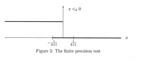
Table 2: Feasible RAM operations and their costs The finite precision test $<_{k}$ with precision $k$ can be defined preciselyby
$(X<_{ky})\ni\{$ TRUE $:\Leftrightarrow x<y$
FALSE $: \Leftrightarrow x>y-\frac{1}{k+1}$
for $x,$$’\iota’j\in \mathbb{R},$ $k\in$ N. In other words: if the test $x<_{k}y$
answers
with TRUE, thenalways $x<y$ holds; and if the
answer
is FALSE, then $x>y- \frac{1}{k+1}$ holds. In the smalloverlapping area of uncertainty of length $\frac{1}{k+1}$ the answer of the test might be TRUE
as
well as FALSE (cf. Figure 3). The reader should notice that the costs of the testoperation increase if the length $\frac{1}{k+1}$ of the overlapping area decreases. For complexity
reasons
we will also use a finite precision staircase operation, giving one of the values in$x$
Figure 3: The finite precision test
It isanimportantobservation that the finiteprecisiontest introducesan indeterminism into our feasible real RAM. More formally, a feasible real RAM computes a relation
$R_{M}\subseteq X\cross Y$ where $(x, y)\in R_{M}$ if there is some computation path on input $x$ with
output $y$. Here, $X,$$Y$ denote finite products of $\mathrm{N}$ and $\mathbb{R}$. But in contrast to the kind of
nondeterminism which is used in complexity theory,
our
indeterminismcan
be realizedon physical machines. Indeterminism and nondeterminismhave in
common
that a single input does potentially lead to several computation paths. While nondeterminism meansthat only some computation paths have to lead to a “valid result”, indeterminism
means
that all computation paths have to lead toa $‘\langle \mathrm{v}\mathrm{a}\mathrm{l}\mathrm{i}\mathrm{d}$
result”. Thus, nondeterminism comes
with an existential quantification and indeterminism with an universal quantification in the definition of semantics. To make this more precise we define our approximative
semantics.
Definition 3.1 (Approximative semantics) Let $M$be a feasiblereal RAM
with
inputspace $X\cross \mathrm{N}$ and output space $Y$ and let $f:\subseteq Xarrow Y,$ $t:\subseteq X\mathrm{x}\mathrm{N}arrow \mathrm{N}$ be functions.
Then $M$ is said to approximate$f$ in time $t$ if$dom(f)\cross \mathrm{N}\subseteq \mathrm{d}\mathrm{o}\mathrm{m}(R_{M})$ and
(1) $d(f(x), y)<2^{-n}$ for all $(x, n)\in \mathrm{d}\mathrm{o}\mathrm{m}(f)\cross \mathrm{N}$and $y\in R_{M}(x, n)$,
(2) $t_{M}(x, n)\leq t(x, n)$ for all $(x, n)\in \mathrm{d}\mathrm{o}\mathrm{m}(f)\cross$ N.
Here $d$ denotes the maximum metric on $Y$, where $Y$ is a finite product of the spaces
$\mathrm{N},$ $\mathbb{R}$ which are equipped with the discrete metric, Euclidean metric, respectively.
Fur-thermore, $t_{M}:\subseteq X\mathrm{x}\mathrm{N}arrow \mathrm{N}$ denotes the logarithmic time complexity of the feasible real
RAM $M$ which can be defined by
$t_{M}(x,$$n)$ $:=$ comp.
$\max_{\mathrm{p}\mathrm{a}\mathrm{t}\mathrm{h}\mathrm{s}\mathrm{o}\mathrm{n}}(x,n)\{\sum \mathrm{c}\mathrm{o}\mathrm{s}\mathrm{t}(op)\}$
$op$
for $(x, n)\in \mathrm{d}\mathrm{o}\mathrm{m}(R_{M})$ where the last sum is over all operations $op$ in a computation path
on input $(x, n)$ and the maximum is over allcomputation paths on input $(x, n)$. Thus, the
logarithmic time complexity measure charges each operation with costs depending onthe size of the operands. Now we are prepared to define time complexity classes for feasible
real RAMs. For $t:\subseteq X\cross \mathrm{N}arrow \mathrm{N}$ we define
$\mathrm{T}\mathrm{I}\mathrm{M}\mathrm{E}_{\mathrm{R}\mathrm{A}\mathrm{M}}(t):=\{f$ $:\subseteq Xarrow Y|Y$ is a finite product of$\mathrm{N}$ and $\mathbb{R}$ and there is
Our main result in this section will compare these time complexity classes with the cor-responding time complexity classes for Turing machines. We recall the fact that in
com-putable analysis the time complexity of a function
measures
the number of Turingma-chinesteps whichare usedinorderto produce the result with precision$2^{-n}$ (cf. Ko [Ko91],
M\"uller $[\mathrm{M}\ddot{\mathrm{u}}186]$, Weihrauch [WeiOO]$)$. Thus, a function $f:\subseteq Xarrow Y$ is in $\mathrm{T}\mathrm{I}\mathrm{M}\mathrm{E}_{\mathrm{T}\mathrm{M}}(t)$ if
and only if there is a Turing machine $M$ which computes $f$ with respect to the binary
signed-digit representation and which produces an approximation of $f(x)$ with precision $2^{-n}$ for each input sequence$p$ which represents $x$ in at most $t(x, n)$ steps. Precise
defini-tions can be found in [BH98]. Now our main result can be stated as follows.
Theorem 3.2 (Feasible real RAM) For regular time bounds $t:\subseteq X\cross \mathrm{N}arrow \mathrm{N}$ the
following inclusion holds: $\mathrm{T}\mathrm{I}\mathrm{M}\mathrm{E}_{\mathrm{T}\mathrm{M}}(t)\subseteq \mathrm{T}\mathrm{I}\mathrm{M}\mathrm{E}_{\mathrm{R}\mathrm{A}\mathrm{M}}(t)\subseteq \mathrm{T}\mathrm{I}\mathrm{M}\mathrm{E}_{\mathrm{T}\mathrm{M}}(t^{2}\cdot\log(t)\cdot\log\log(t))$. Here a time bound$t:\subseteq X\cross \mathrm{N}arrow \mathrm{N}$iscalled regular, if$P(x)+k+t(x, k+1)\subseteq \mathcal{O}(t(x, k))$
and $t(x, k)\geq 2$. This condition is fulfilled by all time bounds of practical interest. In
other words our result states that feasible real RAMs are a polynomially realistic model of computability and complexity on the real numbers (compared to the Turing machine based model of computable analysis). One of the surprising parts of the result is that is
suffices to usethe logarithmictime complexity
measure
whichonly counts the sizes oftheoperands but which does not
measure
the precision ofthe local RAM operations which is necessary to compute the result.Figure 4: The simulation of a RAM $M$ by a TM
The proof justifies this by the fact that the basic arithmetic operations are online
computable in polynomial time, $\mathrm{i}.\mathrm{e}$. there are polynomial-time Rring machine programs
for these operations such that the output precision is equal to the input precision minus a certain fixed delay depending on the input size. This result can be extended to other
larger classes of (smooth) basic operations like the exponential function or trigonometric
functions (cf. [BH98]).
The main part of the proof which shows that feasible real RAMs
can
be simulated by Turing machines is based on the idea to start the simulation with a fixed input precision$m$ and torestart it again and again with adoubling of the input precision until the output
precision suffices. Because of regularity of the time bounds this doubling of precision will not effect the time complexity substantially. The flowchart in Figure 4 illustrates the idea.
4
Theory of
continuous
data
structures
In the previous section we have
seen
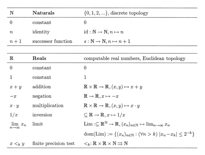
how an abstract description of the model ofcom-putability of computable analysis can be developed, which is realistic with respect to computability and complexity. From a certain point of view we can interpret this
re-sult such that we have found an efficient data structure for real and natural numbers. This data structure can be summarized by the following table (where we have omitted
operations which are not necessary from the point of view of computability).
$\mathrm{N}$ Naturals $\{0,1,2, \ldots\}$, discretetopology
$0$ constant $0$
$n$ identity $\mathrm{i}\mathrm{d}:\mathrm{N}arrow \mathrm{N},$ $n-\rangle$ $n$
$n+1$ successor function $s$ : $\mathrm{N}arrow \mathrm{N},$$n..\mapsto n+1$
$\mathbb{R}$ Reals computable real numbers, Euclidean topology
$0$ constant $0$
1 constant 1
$x+y$ addition $\mathbb{R}\cross \mathbb{R}arrow \mathbb{R},$$(x, y)-,$ $x+y$
$-X$ negation $\mathbb{R}arrow \mathbb{R},$$x-,$ $-x$
$x\cdot y$ multiplication $\mathbb{R}\cross \mathbb{R}arrow \mathbb{R},$$(x, y)-tx\cdot y$
$1/x$ inversion $\subseteq \mathbb{R}arrow \mathbb{R},$$x->1/x$ $\lim_{narrow\infty}x_{n}$ limit Lim
$:\subseteq \mathbb{R}^{\mathbb{N}}arrow \mathbb{R},$ $(x_{n})_{n\in \mathbb{N}}-* \lim_{narrow\infty}x_{n}$
dom(Lim) $:=\{(x_{n})_{n\in \mathbb{N}} : (\forall n>k)|x_{n}-x_{k}|\leq 2^{-k}\}$
$x<_{k}y$ finite precision test $<_{k}$:$\mathbb{R}\cross \mathbb{R}\cross \mathrm{N}=\mathbb{N}$
Of course, in the feasible real RAM the limit operation
was
not an explicit basic operation but it was hidden in the approximative semantics.Inseveral
areas
of computer sciencewedo not only want to compute with realnumbers,but we also want to compute with sets of real numbers and real number functions. In numerical analysis we want for instance transform a program for a continuous function
$f$ : $[0,1]arrow \mathbb{R}$ into a program for its integral function $x-\rangle$ $\int_{0}^{x}f(t)dt$. Or in CAD we
want to compute with compact sets ofrealnumbers and perform operations like the union operation.
Consequently, the question appears how we canfind suitable data structures not only for the real numbers but also for otherspaceslike hyper and function spaces. We just want to mention that an
answer
to this questioncan be givenbythe theory of perfectstructures$[\mathrm{B}\mathrm{r}\mathrm{a}99\mathrm{b}]$. These structures, taken as data structures for a suitable high-level
program-ming language or computability model (like the feasible RAM model) allow to compute exactly the same operations as the Turing machine model together with a correspond-ing representation. Moreover, perfect data structures have the following nice property
$[\mathrm{B}\mathrm{r}\mathrm{a}99\mathrm{c}]$.
Theorem 4.1 (Stability Theorem)
Perfect
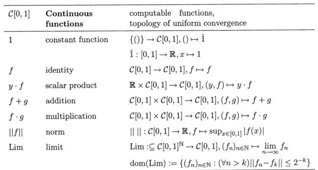
structures characterize their own compu-tability theory.Instead of defining the notion of a perfect structure formally, we just mention two further examples.
$C[0,1]$ Continuous computable functions,
functions topology of uniform convergence
1 constant function $\{()\}arrow C[0,1],$ $()\mapsto\hat{1}$
$\hat{1}$
: $[0,1]arrow \mathbb{R},$ $x\mapsto 1$
$f$ identity $C[0,1]arrow C[0,1],$$f-\rangle f$
$y\cdot f$ scalar product $\mathbb{R}\cross C[0,1]arrow C[0,1],$ $(y, f)-ry\cdot f$
$f+g$ addition $C[0,1]\cross C[0,1]arrow C[0,1],$$(f, g)-tf+g$
$f\cdot g$ multiplication $C[0,1]\cross C[0,1]arrow C[0,1],$$(f, g)rightarrow f\cdot g$
$||f||$ norm $||||$ : $C[0,1]arrow \mathbb{R},$$f-,$ $\sup_{x\in[0,1]}|f(x)|$
Lim limit $\mathrm{L}\mathrm{i}\mathrm{m}:\subseteq C[0,1]^{\mathbb{N}}arrow C[0,1],$
$(f_{n})_{n\in \mathbb{N}} \mapsto\lim_{narrow\infty}f_{n}$
dom(Lim) $:=\{(f_{n})_{n\in \mathbb{N}} : (\forall n>k)||f_{n}-f_{k}||\leq 2^{-k}\}$
Table 4: The structure of continuous functions
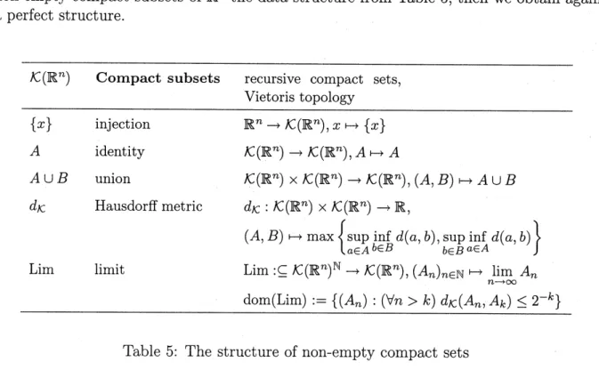
If we add to our data structure of the natural and real numbers the data structure for the space $C[0,1]$ of continuous functions from Table 4 and for the space $\mathcal{K}(\mathbb{R}^{n})$ of
non-empty compact subsets of$\mathbb{R}^{n}$ the data structure from Table 5, then we
obtain again
a perfect structure.
$\mathcal{K}(\mathbb{R}^{n})$ Compact subsets recursive compact sets,
Vietoris topology
$\{x\}$ injection $\mathbb{R}^{n}arrow \mathcal{K}(\mathbb{R}^{n}),$ $x-\rangle\{x\}$
$A$ identity $\mathcal{K}(\mathbb{R}^{n})arrow \mathcal{K}(\mathbb{R}^{n}),$ $Arightarrow A$
$A\cup B$ union $\mathcal{K}(\mathbb{R}^{n})\cross \mathcal{K}(\mathbb{R}^{n})arrow \mathcal{K}(\mathbb{R}^{n}),$$(A, B)-\rangle A\cup B$
$d_{\mathcal{K}}$ Hausdorff metric $d_{\mathcal{K}}$ : $\mathcal{K}(\mathbb{R}^{n})\cross \mathcal{K}(\mathbb{R}^{n})arrow \mathbb{R}$,
$(A, B) \mapsto\max\{\sup_{a\in A}\inf_{b\in B}d(a, b),\sup_{b\in B^{a}}\inf_{\in A}d(a, b)\}$
Lim limit $\mathrm{L}\mathrm{i}\mathrm{m}:\subseteq \mathcal{K}(\mathbb{R}^{n})^{\mathrm{N}}arrow \mathcal{K}(\mathbb{R}^{n}),$
$(A_{n})_{n\in \mathbb{N}}-, \lim_{narrow\infty}A_{n}$
dom(Lim) $:=\{(A_{n}) : (\forall n>k)d_{\mathcal{K}}(A_{n}, A_{k})\leq 2^{-k}\}$
Table 5: The structure of non-empty compact sets
Thus, we have here two possible data $\mathrm{s}\mathrm{t}\mathrm{r}\mathrm{u}\mathrm{c}\dot{\mathrm{t}}\mathrm{u}\mathrm{r}\mathrm{e}\mathrm{s}$
for computations with objects like
compact sets and continuous functions. Of course, these structures represent only
ex-amples of data structures and there are other structures which correspond to different
topologies and computability notions onthe
same
spaces. The tables mention the under-lying topologies and the corresponding sets of computable points.Moreover, the theory of perfect structures can
answer
the question which asks forreasonable data structures only with respect to computability and nothing is said about complexity. For complexity questions, a comprehensive and general theory of computa-tional complexity of metric spaces is still missing.
5
Conclusion
In the introduction we have described the role of the computability model in the cycleof real number programming.
As
the cardinal problem of the real number model we have singled out the discontinuity ofthe comparisons and equality tests. On the on hand, thiscauses a discontinuous description of the problem under consideration and, on the other
hand, this makes a precise implementation on physical computers impossible.
In Section 2 we have presented
some
basic results of computable analysis. Especially,ithas been described preciselywhich computationson the real numbers canbe performed realistically on physical computers. One central result states that only continuous opera-tions can be performed.
In Section 3 we have presented the feasible real RAM model which is an approach to
describe the results of computable analysis in terms which are as close as possible to the
real number model.
In Section4 we have shown, at least onthe level of computability, how these ideas can
be transferred to computations with other objects like compact subsets and continuous functions.
Finally, we propose to replace the original real number model in the cycle of real
number programming by the feasible real RAM model. Such a substitution would have several advantages: ontheone hand, real world problems, especially iftheyareinspiredby
physical questions, are typically continuous. These problemscanbe described pretty good by the continuous (but indeterministic!) feasible real RAM model. On the other hand and maybe more important, each correct algorithm, developed for the feasible real RAM
model, can be implemented on physical computers without any instability or degeneracy
problems!
References
[BH98] Vasco Brattka and Peter Hertling. Feasible real random access machines. Journal of Com-plexity, $14(4):490-526$, 1998.
[BMS94] Christoph Burnikel, Kurt Mehlhorn, and Stefan Schirra. On degeneracy in geometric compu-tations. In Proceedings ofthe
Fifth
Annual $ACM$-SIAMSymposium on Discrete Algorithms($Arlington_{f}$ VA, 1994), pages 16-23, NewYork, 1994. ACM.
[Bra99a] Vasco Brattka. The emperor’s new recursiveness. preprint, 1999.
[Bra99b] Vasco Brattka. Recursive and computable operations over topological structures. Informatik Berichte 255, FernUniversit\"atHagen, FachbereichInformatik, Hagen, July1999. Dissertation. [Bra99c] Vasco Brattka. Astabilitytheorem for recursive analysis. In Cristian S. Calude and Michael J. Dinneen, editors, Combinatorics, Computation $\not\in y$Logic, Discrete Mathematics and
Theoreti-cal Computer Science, pages 144-158, Singapore, 1999. Springer. Proceedings of DMTCS’99 and CATS’99, Auckland, New Zealand, January 1999.
[BSS89] Lenore Blum, Mike Shub, and Steve Smale. On a theory of computation and complexityover
the real numbers: $NP$-completeness, recursive functions and universal machines. Bulletin of
the American Mathematical Society, 21 (1): 1-46, July 1989.
[Grz57] Andrzej Grzegorczyk. Onthedefinitions of computable real continuous functions. Fundamenta
Mathematicae, 44:61-71, 1957.
[Hau73] J\"urgen Hauck. Berechenbare reelle Funktionen. Zeitschrifl f\"ur mathematische Logik und Grundlagen der Mathematik, 19:121-140, 1973.
[HW94] Peter Hertling and KlausWeihrauch. Levels of degeneracy and exact lower complexitybounds
for geometric algorithms. InProceedings ofthe Sixth Canadian Conference on Computational Geometry, pages 237-242. University of Saskatchewan, 1994. Saskatoon, Saskatchewan,
Au-gust 2-6, 1994.
[Ko91] Ker-I Ko. Complexity Theory ofReal Functions. Progress in Theoretical Computer Science. Birkh\"auser, Boston, 1991.
[KW84] Christoph Kreitz and Klaus Weihrauch. A unified approach to constructive and recursive analysis. In M.M. Richter, E. B\"orger, W. Oberschelp, B. Schinzel, and W. Thomas, editors, Computation andProofTheory, volume 1104ofLectureNotes in Mathematics, pages 259-278, Berlin, 1984. Springer. Proceedings of the Logic Colloquium, Aachen, July 18-23, 1983, Part
II.
[Lac55] Daniel Lacombe. Extensionde la notion defonctionr\’ecursive auxfonctionsd’uneouplusieurs variablesr\’eelles I. Comptes Rendus Acad\’emie des Sciences Paris, 240:2478-2480, June 1955.
The’orie des fonctions.
$[\mathrm{M}\ddot{\mathrm{u}}186]$ Norbert Th.M\"uller. Computational complexity of real functions and real numbers. Informatik
Berichte 59, $\dot{\mathrm{F}}\mathrm{e}\mathrm{r}\mathrm{n}\mathrm{U}\mathrm{n}\mathrm{i}\mathrm{v}\mathrm{e}\mathrm{r}\mathrm{s}\mathrm{i}\mathrm{t}\ddot{\mathrm{a}}\mathrm{t}$
Hagen, Hagen, June 1986.
[PER89] MarianB. Pour-El and J. Ian Richards. ComputabilityinAnalysis and Physics. Perspectives in Mathematical Logic. Springer, Berlin, 1989.
[PS85] Franco P. Preparata and Michael Ian Shamos. Computational Geometry. Texts and
Mono-graphs in Computer Science. Springer, NewYork, 1985.
[Tur36] AlanM. Turing. Oncomputable numbers, withanapplication tothe “Entscheidungsproblem”. Proceedings ofthe London Mathematic$al$Society, 42$(.2):230-265$, 1936.
[Tur37] AlanM.Turing. On computable numbers, with an applicationtothe “Entscheidungsproblem”.
A correction. Proceedings ofthe London Mathematical Society, $43(2):544-546$, 1937.
[TWW88] Joseph F. Traub, $\mathrm{G}.\mathrm{W}$. Wasilkowski, and H. Woz’niakowski.
Information-Based
Complexity. Computer Science and Scientific Computing. AcademicPress, New York, 1988.[Wei98] Klaus Weihrauch. A refined model of computation for continuous problems. Journal of Complexity, 14:102-121, 1998.
[WeiOO] Klaus Weihrauch. An Introduction to Computable Analysis. Springer, Berlin, 2000. (to appear).