END-TO-END FEEDBACK LOSS IN SPEECH CHAIN FRAMEWORK VIA STRAIGHT-THROUGH ESTIMATOR

END-TO-END FEEDBACK LOSS IN SPEECH CHAIN FRAMEWORK VIA STRAIGHT-THROUGH ESTIMATOR

Andros Tjandra ^1,2 , Sakriani Sakti ^1,2 , Satoshi Nakamura ^1,2

1 Nara Institute of Science and Technology, Japan

2 RIKEN, Center for Advanced Intelligence Project AIP, Japan {andros.tjandra.ai6,ssakti,s-nakamura}@is.naist.jp

ABSTRACT

The speech chain mechanism integrates automatic speech recogni- tion (ASR) and text-to-speech synthesis (TTS) modules into a single cycle during training. In our previous work, we applied a speech chain mechanism as a semi-supervised learning. It provides the abil- ity for ASR and TTS to assist each other when they receive unpaired data and let them infer the missing pair and optimize the model with reconstruction loss. If we only have speech without transcrip- tion, ASR generates the most likely transcription from the speech data, and then TTS uses the generated transcription to reconstruct the original speech features. However, in previous papers, we just limited our back-propagation to the closest module, which is the TTS part. One reason is that back-propagating the error through the ASR is challenging due to the output of the ASR being discrete tokens, creating non-differentiability between the TTS and ASR.

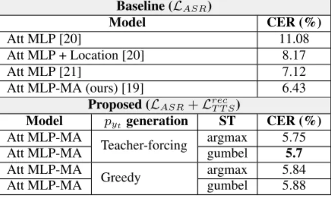
In this paper, we address this problem and describe how to thor- oughly train a speech chain end-to-end for reconstruction loss us- ing a straight-through estimator (ST). Experimental results revealed that, with sampling from ST-Gumbel-Softmax, we were able to up- date ASR parameters and improve the ASR performances by 11%

relative CER reduction compared to the baseline.

Index Terms— speech chain, end-to-end feedback loss, straight- through estimator, ASR, TTS

1. INTRODUCTION

A speech chain [1] is a viewpoint that describes the speech com- munication process in which the speaker produces words and gen- erates speech sound waves, transmits the speech waveform through a medium (i.e., air), and creates a speech perception process in a listeners auditory system to perceive what was said. The hearing process is critical, not only for the listener but also for the speaker herself. By simultaneously listening and speaking, the speaker can monitor her volume, articulation, and the general comprehensibility of her speech. Based on those observations, we simulated the speech chain mechanism by coupling ASR and TTS and formed a machine speech chain [2, 3], so that the machine can learn, not only to lis- ten (by way of ASR) or speak (by way of TTS) but also listen while speaking.

In our previous paper [2], we utilized the speech chain idea for semi-supervised learning using paired and unpaired data. First, we pretrained both ASR and TTS with a small amount of paired speech and text data. Then, we subsequently used both the pretrained mod- ules to complete the missing pair from the unpaired data. For ex- ample, if we only have speech without transcription, ASR generates the most likely transcription from the speech data with greedy or beam-search decoding, and TTS uses the generated transcription to reconstruct the original speech features. In this case, we trained the TTS module with the reconstruction loss. For the reverse case, if

we only have text without any corresponding speech, TTS generates speech, whose features ASR uses to reconstruct the original text. In this case, we updated the ASR module with the reconstruction loss.

In Fig. 1(a), we illustrate a multispeaker speech chain loop between the ASR and TTS modules.

However, the auditory feedback in a human speech chain hap- pens almost constantly, not only during semi-supervised learning.

Furthermore, the close-loop feedback is also done end to end. But, to simulate our speech chain mechanism to provide the ability to help each other even during the supervised learning and perform a com- pletely end-to-end feedback reconstruction loss, the main challenge is to utilize TTS to improve our ASR module. One reason is that back-propagating the error from the reconstruction loss through the ASR module is challenging due to the output of the ASR discrete to- kens (grapheme or phoneme), creating non-differentiability between the TTS and ASR modules (Fig. 1(b)).

We address this problem using a straight-through estimator [4, 5]

to predict the gradient through discrete variables (Fig. 1(c)). We mainly focus on describing how to thoroughly train a speech chain end-to-end by adding a reconstruction term from the TTS module and backpropagated the gradient through the ASR. Experimental re- sults revealed that, with teacher-forcing and sampling from Gumbel- Softmax, we are now able to updated ASR parameters and improved the ASR performances significantly by 11% relative CER reduction compared to the baseline.

2. SPEECH CHAIN AND END-TO-END FEEDBACK LOSS In the speech chain mechanism, given speech features x = [x

1

, .., x

S

] (e.g., Mel-spectrogram) and text y = [y

1

, .., y

T

], we feed the speech to the ASR module, and the ASR decoder generates contin- uous vector h

^d_t

step-by-step. To calculate probability vector p

y

= [p

y₁

, .., p

y_T

], we apply the softmax function p

y_t

= softmax(h

^dt

) to decoder output h

^d_t

. For each class probability mass in p

y_t

, p

y_t

[c]

was defined as:

p

y_t

[c] = exp(h

^d_t

[c]/τ) P

C

i=1

exp(h

^d_t

[i]/τ) , ∀c ∈ [1..C]. (1) Here C is the total number of classes, h

^dt

∈ R

^C

are the logits pro- duced by the last decoder layer, and τ is the temperature parame- ters. Setting temperature τ using a larger value (τ > 1) produces a smoother probability mass over classes [6].

For the generation process, we generally have two different methods:

1. Conditional generation given ground-truth (teacher-forcing):

If we have paired speech and text (x, y), we can generate p

yt

from autoregressive ASR decoder Dec

ASR

(y

t−1

, h

^e

), con-

ditioned to ground-truth text y

t−1

in the current time-step and

Fig. 1. a) Multispeaker machine speech chain mechanism; b) Baseline ([3]): feedback loss from TTS is only backpropagated through the TTS module, and the ASR module is not updated because variable y ˆ is non-differentiable; c) Proposal: feedback loss from TTS is backpropagated through discrete variable y, and ASR modules are updated based on the estimated gradient from the TTS module by a straight-through ˆ estimator.

encoded speech feature h

^e

= Enc

ASR

(x). At the end, the length of probability vector p

y

is fixed to T time-steps.

2. Conditional generation given previous step model prediction:

Another generation process to decode ASR transcription uses its own prediction to generate probability vector p

y_t

. There are many different generation methods, such as greedy de- coding (1-best beam-search) ( y ˜

t

= argmax

c

p

y_t

[c]), beam- search, or stochastic sampling (˜ y

t

∼ Cat(p

y_t

)).

After the generation process, we obtained probability vector p

y

and applied discretization from continuous probability vector p

y_t

to y ˜

t

either by taking the class with the highest probability or sam- pling from a categorical random variable. After getting a single class to represent the probability vector, we encode it into vec- tor [0, 0, .., 1, ..,0] with one-hot encoding representation and give it to the TTS as the encoder input. The TTS reconstructs Mel- spectrogram ˆ x with the teacher-forcing approach. The reconstruc- tion loss is calculated:

L

^recT T S

= 1 S

S

X

s=1

(x

s

− x ˆ

s

)

²

, (2) where x ˆ

s

is the predicted (or reconstructed) Mel-spectrogram and x

s

is the ground-truth spectrogram at s-th time-step.

We directly calculated the gradient from the reconstruction loss w.r.t TTS parameters (∂L

^recT T S

/∂θ

T T S

) because all the operations inside the TTS module are continuous and differentiable. However, we could not calculate the gradient from the reconstruction loss w.r.t ASR parameters (∂L

^recT T S

/∂θ

ASR

) because we have a discretiza- tion operation from p

yt

→ onehot(˜ y

t

). Therefore, we applied a straight-through estimator to enable the loss from L

^recT T S

to pass through discrete variable y ˜

t

.

2.1. Straight-through Argmax

The straight-through estimator [4, 5] is a method for estimating or propagating gradients through stochastic discrete variables. Its main idea is to backpropagate through discrete operations (e.g., argmax

c

p

yt

[c] or sampling y ˜

t

∼ Cat(p

yt

)) like an identity func- tion. We describe the forward process and the gradient calculation with a straight-through estimator in Fig. 2.

In the implementation, we created a function with different for- ward and backward operations. For argmax one-hot encoding func- tion, we formulated the forward operation:

Fig. 2. Straight-through estimator on arg max function. Given input x and model parameters θ, we calculate categorical proba- bility mass P (x; θ) and apply discrete operation argmax. In the backward pass, the gradient from stochastic node y to P (x; θ),

∂y/∂P (x; θ) ≈ 1 is approximated by identity.

˜

z

t

= argmax

c

p

y_t

[c] (3)

˜

y

t

= onehot(˜ z

t

). (4) Here we describe y ˜

t

as a one-hot encoding vector with the same length as the p

y_t

vector. When the loss is calculated and the gra- dients are backpropagated from loss L

^rec_{T T S}

, we formulate the back- ward operation:

∂ ˜ y

t

∂p

yt

≈ 1. (5)

Therefore, when we back-propagate the loss from Eq. 2 with the straight-through estimator approach, we calculate the TTS recon- struction loss gradient w.r.t θ

ASR

:

∂L

^rec_{T T S}

∂θ

ASR

=

T

X

t=1

∂ L

^rec_{T T S}

∂ y ˜

t

· ∂ y ˜

t

∂p

y_t

· ∂p

yt

∂θ

ASR

(6)

≈

T

X

t=1

∂ L

^recT T S

∂ y ˜

t

· 1 · ∂p

y_t

∂θ

ASR

. (7)

2.2. Straight-through Gumbel Softmax

Besides taking argmax class from probability vector p

y_t

, we also

generated a one-hot encoding by sampling with the Gumbel-Softmax

Fig. 3. Given speech feature x, ASR generates a sequence of proba- bility p

y

= [p

y₁

, p

y₂

, ..., p

y_T

]. If we have a ground-truth transcrip- tion, we can calculate L

ASR

(Eq. 16). TTS module generates speech features, and we calculate reconstruction loss L

^rec_{T T S}

(Eq. 2). After that, the gradients based on L

ASR

are propagated through the ASR module, and the gradients based on L

^rec_{T T S}

are propagated through the TTS and ASR modules by a straight-through estimator.

distribution [7, 8]. Gumbel-Softmax is a continuous distribution that approximates categorical samples, and the gradients can be calcu- lated with a reparameterization trick. For Gumbel-Softmax, we re- placed the softmax formula for calculating p

y_t

(Eq. 1):

p

y_t

[c] = exp((h

^dt

[c] + g

c

)/τ ) P

C

i=1

exp((h

^d_t

[i] + g

i

)/τ ) , ∀c ∈ [1..C]. (8) where g

1

, .., g

C

are i.i.d samples drawn from Gumbel(0, 1) and τ is the temperature. We sample g

c

by drawing samples from the uniform distribution:

u

c

∼ Uniform(0, 1) (9) g

c

= − log(− log(u

c

)), ∀c ∈ [1..C]. (10) To generate a one-hot encoding, we define our forward operation:

˜

z

t

∼ Categorical(p

yt

[1], p

yt

[2], ..., p

yt

[C]) (11)

˜

y

t

= onehot(˜ z

t

). (12) At the backpropagation time, we use the same straight-through es- timator (Eq. 5) to allow the gradients to flow through the discrete sampling operation from Eq. 11.

2.3. Combined Loss for ASR

Our final loss function for ASR is a combination from negative likeli- hood (Eq. 16) and TTS reconstruction loss (Eq. 2) by sum operation:

L

^FASR

= L

ASR

+ L

^recT T S

. (13) To summarize our explanation in this section, we provide an illus- tration in Fig. 3 that explains how sub-losses L

ASR

and L

^recT T S

are backpropagated to the rest of the ASR and TTS modules.

3. SEQUENCE-TO-SEQUENCE MODEL FOR ASR A sequence-to-sequence model is a neural network that directly models conditional probability p(y|x), where x = [x

1

, ..., x

S

] is the sequence of the (framed) speech features with length S and y = [y

1

, ..., y

T

] is the labels sequence with length T .

The encoder task processes input sequence x and generating rep- resentative information h

^e

= [h

^e₁

, ..., h

^e_S

] for the decoder. The atten- tion module is an extension scheme that assists the decoder to find relevant information on the encoder side based on the current de- coder hidden states h

^d_t

[9, 10]. Attention modules produce context information c

t

at time t based on the encoder and decoder hidden states:

c

t

=

S

X

s=1

a

t

(s) ∗ h

^es

(14)

a

t

(s) = Align(h

^es

, h

^dt

)

= exp(Score(h

^e_s

, h

^d_t

)) P

S

s=1

exp(Score(h

^e_s

, h

^d_t

)) . (15) There are several variations for score functions [11] such as Score(h

^es

, h

^dt

): dot product (hh

^es

, h

^dt

i), bilinear (h

^e|s

W

s

h

^dt

), where Score : ( R

^M

× R

^N

) → R , M is the number of hidden units for the encoder and N is the number of hidden units for the decoder.

Finally, the decoder task predicts target sequence probability p

y_t

at time t based on previous output and context information c

t

. The loss function for ASR can be formulated:

L

ASR

= − 1 T

T

X

t=1 C

X

c=1

1 (y

t

= c) ∗ log p

y_t

[c], (16)

where C is the number of output classes. Input x for the speech recognition tasks is a sequence of feature vectors like a Mel-scale spectrogram. Therefore, x ∈ R

^S×D

, where D is the number of features and S is the total frame length for an utterance. Output y, which is a speech transcription sequence, can be either a phoneme or a grapheme (character) sequence.

4. SEQUENCE-TO-SEQUENCE MODEL FOR TTS Speech synthesis can be viewed as a sequence-to-sequence task where a model generates speech given a sentence. We directly model the conditional probability p(x|y) with a sequence-to-sequence model, where y = [y

1

, ..., y

T

] is the sequence of characters with length T and x = [x

1

, ..., x

S

] is the sequence of (framed) speech features with length S. From the sequence-to-sequence ASR model perspective, TTS is the reverse case where the model reconstructs the original speech given the text.

In this work, our core architecture is based on Tacotron [12] with several structural modifications [3]. The main difference between our modified Tacotron and the default Tacotron is that we added an additional speaker embedding projection layer into our decoder to enable multispeaker training and generation. We also have an addi- tional output layer to generate binary prediction b

s

∈ [0, 1] (1 if the s-th frame is the end of speech, otherwise 0).

For training the TTS model, we used the following loss function:

L

T T S

= 1 S

S

X

s=1

(x

^Ms

− x ˆ

^Ms

)

²

+ (x

^Rs

− x ˆ

^Rs

)

²

− (b

s

log(ˆ b

s

) + (1 − b

s

) log(1 − ˆ b

s

)), (17)

where x ˆ

^M

, x ˆ

^R

, ˆ b are the predicted log Mel-scale spectrogram, the log magnitude spectrogram, and the end-of-frame probability, and x

^M

, x

^R

, b is the ground-truth. In the decoding process, we use the Griffin-Lim algorithm [13] to iteratively estimate the phase spectro- gram and reconstruct the signal with inverse STFT.

5. EXPERIMENT 5.1. Dataset

We evaluated the performance of our proposed method on the Wall Street Journal dataset [14]. Our settings for the training, develop- ment, and test sets are the same as the Kaldi s5 recipe [15]. We trained our model with WSJ-SI284 data. Our validation set was dev 93, and our test set was eval 92.

We used the character sequence as our decoder target and fol- lowed the preprocessing steps proposed by a previous work [16].

The text from all the utterances was mapped into a 32-character set:

26 (a-z) letters of the alphabet, apostrophes, periods, dashes, space, noise, and “eos.” In all the experiments, we extracted the 40 dims +

∆ + ∆∆ (total 120 dimensions) log Mel-spectrogram features from our speech and normalized every dimension into zero mean and unit variance.

5.2. Model Details

For the ASR model, we used a standard sequence-to-sequence model with an attention module (Section 3). On the encoder sides, the input log Mel-spectrogram features were processed by three bidirectional LSTMs (Bi-LSTM) with 256 hidden units for each LSTM: a total of 512 hidden units for the Bi-LSTM. To reduce the memory consump- tion and processing time, we used hierarchical sub-sampling [17, 18]

on all three Bi-LSTM layers and reduced the sequence length by a factor of eight. On the decoder sides, we projected one-hot encoding from the previous character into a 256-dims continuous vector with an embedding matrix, followed by one unidirectional LSTM with 512 hidden units. For the attention module, we used the content- based attention + multiscale alignment (denoted as “Att MLP-MA”) [19] with a 1-history size. In the evaluation stage, the transcription was generated by beam-search decoding (size=5), and we normal- ized the log-likelihood score by dividing it with its own length to prevent the decoder from favoring shorter transcriptions. We did not use any language model or lexicon dictionary in this work. In the training stage, we tried ST-argmax (Section 2.1) and ST-gumbel soft- max (Section 2.2). We also tried both teacher-forcing and greedy de- coding to generate ASR probability vectors p

y

in the training stage.

For each scenario, we treated temperature τ = [0.25, 0.5, 1, 2] as our hyperparameter and searched for the best temperature based on the CER (character error rate) on the development set.

For the TTS model, we used the TTS explained in Section 4.

The hyperparameters for the basic structure are generally the same as those for the original Tacotron, except we replaced ReLU with the LReLU function. For the CBHG module, we used K = 8 fil- ter banks instead of 16 to reduce the GPU memory consumption.

For the decoder sides, we deployed two LSTMs instead of a GRU with 256 hidden units. For each time-step, our model generated four consecutive frames to reduce the number of steps in the decoding process.

5.3. Experiment Result

For our baseline, we trained an encoder-decoder with MLP + mul- tiscale alignment with a 1-history size [19]. We also added several

Table 1. ASR experiment result on WSJ dataset test eval92.

Baseline (L

ASR

)

Model CER (%)

Att MLP [20] 11.08

Att MLP + Location [20] 8.17

Att MLP [21] 7.12

Att MLP-MA (ours) [19] 6.43

Proposed (L

ASR

+ L

^rec_{T T S}

)

Model p

yt

generation ST CER (%)

Att MLP-MA argmax 5.75

Att MLP-MA Teacher-forcing

gumbel 5.7

Att MLP-MA argmax 5.84

Att MLP-MA Greedy

gumbel 5.88

published results to our baseline. All of the baseline models were trained by minimizing negative log-likelihood L

ASR

(Eq. 16).

All the models in the proposed section were trained with a com- bination from two losses: L

ASR

+ L

^rec_{T T S}

, and the ASR parameters were updated based on the gradient from the sum of the two losses.

We have four different scenarios, most of which provide significant improvement compared to the baseline model that is only trained on L

ASR

loss. With teacher-forcing and sampling from Gumbel- softmax, we obtained 11% relative improvement compared to our best baseline Att MLP-MA.

6. RELATED WORKS

Approaches that utilize end-to-end feedback learning from source- to-target and vice-versa remain scant. Senrich et al. [22] improved the NMT performance by back-translation on a monolingual dataset.

Semi-supervised learning for NMT called dual learning [23] was also proposed by combining reconstruction loss and language model reward. However, the feedback gradient provided by the reconstruc- tion loss only limited the closest module to the loss. One primary reason is that the nature of text modalities is represented by discrete variables. Our previous speech chain paper [2, 3] focused on uti- lizing the closed-loop between ASR and TTS as a semi-supervised learning method. If one of the modalities of data is missing, we can generate a pseudo-pair and train one of the models by recon- struction loss. But, as we described earlier, the study also limit the back-propagation to the closest module due to similar reason that the output of the ASR is discrete tokens. In contrast, in this paper, we successfully address the problem using a straight-through estimator to predict the gradient through discrete variables.

7. CONCLUSIONS

We introduced a different perspective from a speech chain mecha- nism. We trained our ASR module by adding feedback from the TTS reconstruction loss. However, the ASR output is not differ- entiable because of the transcription generated by the discretization process. To address this problem, we used a straight-through esti- mator to enable the gradient from the TTS module to flow through discrete variables. We tried various scenarios with different decod- ing and discretization processes. From our experimental results, with teacher-forcing and sampling from Gumbel-Softmax, we improved the ASR performances by 11% relative CER reduction compared to our baseline.

8. ACKNOWLEDGMENT

Part of this work was supported by JSPS KAKENHI Grant Numbers

JP17H06101 and JP17K00237.

9. REFERENCES

[1] P.B. Denes and E. Pinson, The Speech Chain, Anchor books.

Worth Publishers, 1993.

[2] A. Tjandra, S. Sakti, and S. Nakamura, “Listening while speaking: Speech chain by deep learning,” in 2017 IEEE Automatic Speech Recognition and Understanding Workshop (ASRU), Dec 2017, pp. 301–308.

[3] Andros Tjandra, Sakriani Sakti, and Satoshi Nakamura, “Ma- chine speech chain with one-shot speaker adaptation,” in In- terspeech 2018, 19th Annual Conference of the International Speech Communication Association, Hyderabad, India, 2-6 September 2018., 2018, pp. 887–891.

[4] Yoshua Bengio, Nicholas L´eonard, and Aaron Courville, “Es- timating or propagating gradients through stochastic neurons for conditional computation,” arXiv preprint arXiv:1308.3432, 2013.

[5] Geoffrey Hinton, “Neural networks for machine learning, Coursera video lectures,” 2012.

[6] Geoffrey Hinton, Oriol Vinyals, and Jeff Dean, “Distill- ing the knowledge in a neural network,” arXiv preprint arXiv:1503.02531, 2015.

[7] Eric Jang, Shixiang Gu, and Ben Poole, “Categorical reparam- eterization with gumbel-softmax,” 2017.

[8] Chris J Maddison, Andriy Mnih, and Yee Whye Teh, “The con- crete distribution: A continuous relaxation of discrete random variables,” arXiv preprint arXiv:1611.00712, 2016.

[9] Dzmitry Bahdanau, Kyunghyun Cho, and Yoshua Bengio,

“Neural machine translation by jointly learning to align and translate,” arXiv preprint arXiv:1409.0473, 2014.

[10] William Chan, Navdeep Jaitly, Quoc Le, and Oriol Vinyals,

“Listen, attend and spell: A neural network for large vocabu- lary conversational speech recognition,” in Acoustics, Speech and Signal Processing (ICASSP), 2016 IEEE International Conference on. IEEE, 2016, pp. 4960–4964.

[11] Minh-Thang Luong, Hieu Pham, and Christopher D Manning,

“Effective approaches to attention-based neural machine trans- lation,” arXiv preprint arXiv:1508.04025, 2015.

[12] Yuxuan Wang, RJ Skerry-Ryan, Daisy Stanton, Yonghui Wu, Ron J Weiss, Navdeep Jaitly, Zongheng Yang, Ying Xiao, Zhifeng Chen, Samy Bengio, et al., “Tacotron: A fully end-to-end text-to-speech synthesis model,” arXiv preprint arXiv:1703.10135, 2017.

[13] Daniel Griffin and Jae Lim, “Signal estimation from modified short-time fourier transform,” IEEE Transactions on Acoustics, Speech, and Signal Processing, vol. 32, no. 2, pp. 236–243, 1984.

[14] Douglas B Paul and Janet M Baker, “The design for the wall street journal-based csr corpus,” in Proceedings of the work- shop on Speech and Natural Language. Association for Com- putational Linguistics, 1992, pp. 357–362.

[15] Daniel Povey, Arnab Ghoshal, Gilles Boulianne, Lukas Bur- get, Ondrej Glembek, Nagendra Goel, Mirko Hannemann, Petr Motlicek, Yanmin Qian, Petr Schwarz, Jan Silovsky, Georg Stemmer, and Karel Vesely, “The Kaldi speech recognition toolkit,” in IEEE 2011 Workshop on Automatic Speech Recog- nition and Understanding. Dec. 2011, IEEE Signal Processing Society, IEEE Catalog No.: CFP11SRW-USB.

[16] Awni Y Hannun, Andrew L Maas, Daniel Jurafsky, and An- drew Y Ng, “First-pass large vocabulary continuous speech recognition using bi-directional recurrent DNNs,” arXiv preprint arXiv:1408.2873, 2014.

[17] Alex Graves, “Supervised sequence labelling,” in Supervised Sequence Labelling with Recurrent Neural Networks, pp. 5–13.

Springer, 2012.

[18] Dzmitry Bahdanau, Jan Chorowski, Dmitriy Serdyuk, Phile- mon Brakel, and Yoshua Bengio, “End-to-end attention-based large vocabulary speech recognition,” in Acoustics, Speech and Signal Processing (ICASSP), 2016 IEEE International Confer- ence on. IEEE, 2016, pp. 4945–4949.

[19] Andros Tjandra, Sakriani Sakti, and Satoshi Nakamura,

“Multi-scale alignment and contextual history for attention mechanism in sequence-to-sequence model,” To appear in IEEE SLT 2018, 2018.

[20] Suyoun Kim, Takaaki Hori, and Shinji Watanabe, “Joint ctc-attention based end-to-end speech recognition using multi- task learning,” in Acoustics, Speech and Signal Process- ing (ICASSP), 2017 IEEE International Conference on. IEEE, 2017, pp. 4835–4839.

[21] Andros Tjandra, Sakriani Sakti, and Satoshi Nakamura,

“Attention-based wav2text with feature transfer learning,” in 2017 IEEE Automatic Speech Recognition and Understand- ing Workshop, ASRU 2017, Okinawa, Japan, December 16-20, 2017, 2017, pp. 309–315.

[22] Rico Sennrich, Barry Haddow, and Alexandra Birch, “Improv- ing neural machine translation models with monolingual data,”

in Proceedings of the 54th Annual Meeting of the Association for Computational Linguistics (Volume 1: Long Papers), 2016, vol. 1, pp. 86–96.

[23] Di He, Yingce Xia, Tao Qin, Liwei Wang, Nenghai Yu, Tieyan

Liu, and Wei-Ying Ma, “Dual learning for machine transla-

tion,” in Advances in Neural Information Processing Systems,

2016, pp. 820–828.