九州大学学術情報リポジトリ
Kyushu University Institutional Repository
ラプラシアン行列と標準カットに基づくグラフ分割 に関する研究
Kahatapiti Kankanamalage Kissani Ridma, Perera
Graduate School of Mathematics, Kyushu University
https://doi.org/10.15017/21705
出版情報:Kyushu University, 2011, 博士(機能数理学), 課程博士 バージョン:
A study on normalized Laplacian, normalized cut and graph partitioning
A Dissertation Submitted to the Graduate School of Mathematics in Fulfillment of the Requirements for the Degree of
Doctor of Philosophy in Functional Mathematics Kyushu University
By
K.K.Kissani Ridma Perera
Supervisor: Associate Professor Yoshihiro Mizoguchi
March 2012
Abstract
In the last decade important relations between the Laplacian eigenvalues and the eigenvectors of graphs and several other graph parameters were discovered. Spectral clustering uses eigenvalues and eigenvectors of matrices associated with graphs to find clusters in the graphs and is widely used to analysis the social networks, web graphs, communication networks etc. In this thesis, we present some of the results and discuss their consequences in spectral clustering and graph energy. We mainly consider normalized Laplacian matrix to find the bipartitions of graphs. Normalized cut introduced by Shi and Malik in 2000 also play a vital role in graph partitioning problems. There is a close relationship between the second smallest eigenvalue of normalized Laplacian matrix and the normalized cut. We compare these two clustering methods and discuss their performances. Besides that we also consider the Laplacian energy of directed graphs, which is also an application of the Laplacian matrices.
First we review the basic terminologies and key results related to Laplacian matrices, which will be used throughout this thesis.
Next we discuss the properties of minimum normalized cut introduced by Shi and Malik for image segmentations. Several authors considered the applications of normalized cut for graph partitioning and less attention is paid for theoretical explanation of this measure compare with isoperimetric and Cheeger constant. Here we use the notationM cut(G) to represent the minimum normalized cut and derive formula for M cut(G) of some basic classes of graphs such as paths, cycles, complete graphs, double trees and cycle cross paths and some complex graphs such as lollipop type graphsLPn,mand LPn,2′ , roach type graphs Rn,k, weighted paths Pn,k and double tree cross paths.
Next we discuss three matrices associated with graphs called difference Laplacian matrix, nor- malized Laplacian matrix and signless Laplacian matrix and review some known results. Specially we discuss the boundary values of the second smallest eigenvalue of the difference and normalized Laplacian matrices using isoperimetric number and Cheeger constant. Then we derive eigenvalues and eigenvectors of difference, normalized and signless Laplacian matrices of paths and cycles using circulant matrices and give an alternative proof for the eigenvalues of an adjacency matrix of paths and cycles using Chebyshev polynomials. Even most of these results are well known results, we try to summarize them, providing uniform proofs in a simple way.
Next we address the problem of finding graphs which perform poorly on spectral methods. In 1973, Fiedler discussed the possibility of graph partitioning using the sign patterns of second eigenvector of difference Laplacian matrix. Fiedler’s investigation was extended by Davies et al. in 2001 using nodal domain theorem. We use the term Lcut(G) to represent the minimum normalized cut of partitions produced by the second eigenvector of normalized Laplacian matrix. Final goal of studyingM cut(G) andLcut(G) is to investigate the cases, where spectral method perform poorly. More precisely, we give counter examples of graphs and conditions, whereM cut(G) andLcut(G) produce different clusters on graphs. Especially, we investigate the graphsRn,k, LPn,m, LPn,2′ and find conditions, where these two measures make different clusters. We also noticed that the second eigenvector of double tree is an odd vector and therefore we always have M cut(DTn) =Lcut(DTn). This is an exception for the counter examples we discussed under this chapter.
Next we address the problem of finding directed graphs with minimum Laplacian energy. First, we define Laplacian energy of a directed graph as the sum of squares of eigenvalues of a Laplacian matrix defined by using outdegrees of vertices. Then we derive a formula for Laplacian energy of a simple directed graph and show that Laplacian energy of directed graphs can be represented as a sum of squares of outdegrees. Then we consider the classP(α) which consists of non isomorphic graphs with energy less than some positive value αand find 47 non isomorphic directed graphs for class P(10).
Since we can represent the Laplacian energy as a sum of squares of outdegrees of vertices, it motivates us to consider the problem of minimizing sum of squares of degrees in order to find the graph with minimum Laplacian energy. Especially, we studied MMO algorithm introduced by Asahiro 2006, to minimize the maximum outdegree of a directed graph and discuss how far it is applicable to solve our problem and give counter examples, where it is failed. Since the Laplacian energy formula, which we derived is a strict convex function, our problem can be solved by finding optimal semi matching in the bipartite graph.
Finally, we demonstrate the experimental results about spectral clustering on directed graphs.
Most real world networks such as network communications, web graphs, social networks etc. are directed and it is worth to analyze the clustering problem in directed graphs. Since a graph con- structed by hyper links in web-pages is a directed graph, its adjacency matrix Ais asymmetric and does not always have real eigenvalues. Therefore we analyzed the appropriateness of the spectral clustering algorithms on directed graphs. We extend the undirected spectral clustering algorithms to directed graphs using the directed Laplacian matrix introduced by Fan Chung in 2005 and k-means algorithms. Then we compare clustering algorithms based on random walk models and symmetrized transformations. Further we propose an algorithm based on merging techniques. First we apply the directed clustering algorithm and find initial k′ number of clusters and then we merge clusters by minimizing normalized cut introduced by Zhou et al. in 2005 for directed graphs until we receive required number of clusters.
Acknowledgments
First, I would like to express my deepest gratitude to Professor Yoshihiro Mizoguchi, my supervisor as well as the academic advisor, for his continues support, valuable guidance, suggestions and en- couragement. I am also grateful to Professor Hiroyuki Ochiai for his valuable suggestions and helpful comments to succeed this research. I would express my gratitude to Professor Tomoyuki Shirai and Professor Hidefumi Kawasaki for their helpful comments and support to complete this research. I am grateful to Dr. Tetsuji Taniguchi of Matsue College of Technology and Dr. Yasunari Fukai of Kyushu University for their valuable comments and suggestions.
I would like to thank my scholarship donorMONBUKAGAKUSHOfor funding my academic expenses and providing a living stipend. Without this scholarship, I may have not realized my achievements in Japan. I would like to extend my gratitude to the President of Kyushu University, the Dean of the Faculty of Mathematics and the Head of the Department of Mathematics for providing me an opportunity to study in Kyushu University as a foreign student. I also express my gratitude to the Vice Chancellor, the Dean of Faculty of Science, the staff of Department of Mathematics of University of Kelaniya, Sri Lanka for providing me an opportunity to have higher studies in Japan.
My wholeheartedly gratitude goes to my parents, specially to my loving father who was the person behind all the success in my life, providing me every support to have a good education. I express my special gratitude to my husband and son, who bear everything during my studies. At last but not least I thanks the Japanese students in my lab, the officials of various academic and non-academic divisions of Kyushu university for their kind support during my studies in the Kyushu University, Japan.
Contents
Abstract i
Acknowledgments iii
1 Introduction 1
1.1 Introduction . . . 1
1.2 Preliminaries . . . 4
1.3 Formal notations for graphs . . . 14
2 Minimum normalized cut of some graph classes 18 2.1 Properties ofM cut(G) . . . . 18
2.2 General properties ofM cut(G) . . . . 20
2.3 M cut(G) of elementary classes of graphs . . . 21
2.4 M cutof weighted pathsPn,k . . . 29
2.5 M cutof graph LPn,m . . . 33
2.6 M cutof graph LPn,2′ . . . 35
2.7 Double tree cross path . . . 36
2.8 Conclusion . . . 41
3 Difference Laplacian, normalized Laplacian, signless Laplacian and their eigenval- ues 42 3.1 Difference Laplacian and bounds for the eigenvalues . . . 42
3.2 Normalized Laplacian . . . 49
3.2.1 Properties of normalized Laplacian . . . 49
3.2.2 Cheeger constant of graphs . . . 54
3.2.3 Bounds for the normalized eigenvalues of paths . . . 58
3.2.4 Bounds for the normalized eigenvalues of weighted paths . . . 60
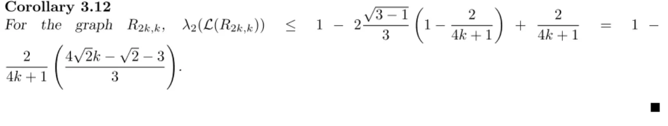
3.2.5 Bounds for the normalized eigenvalues ofR2k,k . . . 60
3.2.6 Normalized eigenvalues of elementary graphs . . . 63
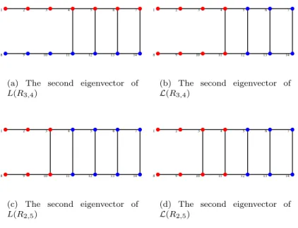
3.2.7 Sign patterns of difference and normalized Laplacian eigenvectors . . . 63
3.3 Signless Laplacian . . . 64
3.3.1 Signless Laplacian eigenvalues of some graphs . . . 65
3.3.2 Properties of signless Laplacian . . . 66
3.4 The eigenvalues and the eigenvectors of paths and cycles . . . 68
3.4.1 Circulant matrices and eigenvalues of cycles and paths . . . 68
3.4.2 Chebyshev polynomials and eigenvalues of adjacency matrix of paths and cycles 76 3.4.3 Determinant of tridiagonal Matrices . . . 78
3.5 Conclusion . . . 81
4 Counter examples for M cut(G)̸=Lcut(G) 82 4.1 Properties ofLcut(G) . . . . 82
4.2 The graphRn,k . . . 85
4.3 The lollipop graphLPn,m . . . 88
4.4 The graphLPn,2′ . . . 97
4.5 Double tree . . . 100
4.6 Conclusion . . . 104
5 Laplacian energy of directed graphs 105 5.1 Introduction . . . 105
5.2 Laplacian energy of undirected graphs. . . 105
5.3 Laplacian energy of directed graphs . . . 107
5.4 Relationship between undirected graphs and directed graphs . . . 110
5.5 Minimizing maximum outdegree algorithms and Laplacian energy . . . 113
5.6 Find an oriented graph with minimum Laplacian energy using semi-matchings . . . 119
5.7 Characterization of optimal semi matchings . . . 119
5.8 Conclusion . . . 124
6 Spectral clustering for directed graphs 125 6.1 Introduction . . . 125
6.2 Spectral clustering on undirected graphs . . . 125
6.3 Experimental results . . . 127
6.4 Random walk on directed graphs . . . 129
6.5 Comparison of clustering methods . . . 132
6.6 Proposed method by using merging techniques . . . 132
6.7 Conclusion . . . 135
References 137
1 Introduction
1.1 Introduction
Clustering is a common technique in multivariate data analysis, data mining, machine learning etc.
The goal of clustering or partitioning problem is to find groups such that entities within the same group are similar and different groups are dissimilar. In the graph partitioning problem much attention is given to seek the precise criteria to obtain a good partition. Clustering methods, which use eigenvalues and eigenvectors of matrices associated with graphs are called spectral clustering and widely used for graph partitioning problems. Specially, eigenvalues and eigenvectors of Laplacian matrices play a vital role in graph partitioning problems. In 1973, Fiedler named the second smallest eigenvalueλ2
of difference Laplacian matrix as the algebraic connectivity of a graph [16]. In 1975, Fiedler showed that we can decompose a connected graph G into two connected components using only the sign structure of an eigenvector related to the second smallest eigenvalue [17]. Fiedler’s investigation was extended by Davies in 2001 using discrete nodal domain theorem [14]. Laplacian matrix, normalized Laplacian matrix and adjacency matrix with negative non diagonal entries can be used with the nodal domain theorem. Nodal domain theorem is useful to identify the number of connected sign graphs of a given graph based on their eigenvectors and eigenvalues. In 1984, Buser investigated the graph invariant quantityi(G) = min
U
cut(U, V \U)
|U| , which considered the relation between the size of the cut and the size of the separated subsetU [8]. He called it the isoperimetric number i(G) and the optimal bisection was given by the minimum i(G). Later in 1991, Mohar surveyed the spectrum of difference Laplacian matrix of graphs with special emphasis on the second smallest difference Laplacian eigenvalues λ2(G) and its relation to numerous graph invariants, including connectivity, expanding properties, isoperimetric number, maximum cut, independent number, genus, diameter, mean distance, and bandwidth-type parameters of a graph [35]. Clustering techniques discussed by Wu and Leahy was based on the network flow theory [47]. Minimum cuts in an undirected adjacency graphs are used for partitioning data on large graphs. However this method can be extended to find the partitions in directed network graphs and it is beyond this papers work.
In 1995, Guattery and Miller considered two spectral separation algorithms that partition the vertices based on the values of their corresponding entries in second eigenvector and provide some counter examples for which each of these algorithms produces poor separators [18, 19]. They used eigenvector based on the second smallest eigenvalue of the difference Laplacian matrix as well as a specified number of eigenvector corresponding to the smallest eigenvalues. Finally they used general- ized version of spectral methods that allow to use more than a constant number of eigenvector and showed that there are some graphs for which any of the above spectral algorithms perform poorly.
We follow their method especially about graph automorphism and even-odd eigenvector theorem for concrete classes of graphs such as roach graphs, double-trees and double tree cross paths. We also describe these properties using formal notations of graphs.
In 1997, Fan Chung discussed most important theories and properties regarding the eigenvalues of normalized Laplacian matrices of graphs and its applications to graph separator problems[10]. She considered partitioning problem using Cheeger constant and derived fundamental relations between eigenvalues and the Cheeger constant. In 2000, Shi and Malik proposed a measure of disassociation called normalized cut for image segmentations [42]. This measure computed the cut cost as a fraction of total edge connections. The normalized cut is used to minimize the disassociation between groups and maximize the association within groups. However minimization of normalized cut criteria is NP
hard. Therefore approximate discrete solutions were given. Solution to the minimization problem of normalized cut was given by the second smallest eigenvector of the generalized eigensystem, (D− W)y =λDy, where D is the diagonal matrix with vertex degrees andW is the weighted adjacency matrix. They used minimum normalized cut value as a splitting point and find bisection using second smallest eigenvector. They also noted that eigenvectors are well separated and this kind of splitting point is very reliable. Normalized cut introduced by Shi and Malik is useful for several areas [42].
This measure become interested not only for image segmentation but also for other authors who are interested in network theories and statistics. In 2001, Andrew et al. analyzed the clustering algorithms introduced by Shi and Malik and provided some conditions under which the algorithms work well using matrix perturbation theory [4]. Normalized cut problems were analyzed by Ying Du et al. and provided an approximation algorithm for the minimum normalized cut problem [15]. The theoretical and empirical insight into the nature of the three partitioning measures called minimum, average and normalized cut in terms of the underlying image statistics has been studied by Soundararajan and Sarkar in 2003 [44]. They showed that the normalized cut can be expressed as a sum of two beta distributed random variables, whose parameters are functions of the partition classes. Recently Saralees Nadarajah [37, 36] studied normalized cut from the statistical point of view and derived expressions for mode of the normalized cut. In this thesis, we review several properties of normalized cut and find concrete formula for minimum normalized cut (M cut(G)) of some classes of graphs even this is a NP-hard problem. We also find counter example graphs, where clustering based on normalized Laplacian and normalized cut perform differently.
Eigenvalues of Laplacian matrices play a vital role in mathematical chemistry. Especially in the area of graph energy. Energy has been studied in mathematical perspective as well as physical per- spective for several years ago by several authors ([32, 13, 20, 27, 26, 7, 22]). Research on the energy concept dated back to 1940. Coulson evaluated the total energy of π electrons in an unsaturated hydrocarbon molecule [12]. Later, this energy is represented by the sum of absolute values of eigen- values of adjacency matrices of molecular structure by Ivan Gutman. At the beginning, attention is paid to adjacency matrices and later eigenvalues of several kinds of matrices have been studied, of which Laplacian matrix attracted the greatest attention. Several criteria related to the energy of graphs such as energy change due to edge addition, maximal energy, equal energy has been considered by [3],[27] and [7]. Since molecular graphs have undirected structure, energy and Laplacian energy concept originally developed for undirected graphs. Recently, few authors considered the energy of directed graphs. In 2009, Adiga et al. considered Laplacian energy of directed graphs using skew Laplacian matrix, in which degree of a vertex is the sum of its outdegree and indegree [2, 1]. They extended undirected Laplacian energy to directed graphs by using energy definitions given by [22] and [28]. Further Song et al. use Laplacian energy to find the semantic structures of the image hierarchies of graph, which is an different approach to arranging communities in directed graphs [43]. Most algorithms are developed to minimize the maximum outdegree or maximize the minimum outdegree of an oriented graph. Here we find oriented graph with minimum sum of squares of outdegrees and our approach is based on the Laplacian energy of directed graphs, which is different from the existing approaches.
Extension of undirected clustering algorithms to directed graphs has been considered by several authors. Most real world networks are directed and it is still an unsolved problem for finding efficient clustering algorithms for the directed graphs. In 1999, Kleinberg introduce the framework called
’authority’ and ’hub’, which separates web page into 2 categories using ranking algorithms, which converges to spectral methods that uses principal eigenvectors of AAT and ATA [25]. Different approach called page rank algorithm is used by the Google search engine introduced by Page et al.
with eigenvectors of A itself [40]. In 2005, Zhou et al. used directed spectral clustering method to separate the university web pages into student pages and non-student pages [50]. They extended the normalized cut introduced by Shi and Malik for image segmentation to directed clustering [42]. They used directed Laplacian to find the 2 clusters by using second eigenvector and then they extend the algorithm up tokclusters by minimizing normalized cut values. Leicht and Newman also introduced a modularity function for directed graphs [29]. They first divide the network into two groups using the second eigenvector of the modularity matrix and then divide those groups further by repeated bisection while maximizing the modularity function. The process stops when they reach a point at which further division does not increase the total modularity of the network. This method always use the second eigenvector of modularity matrix for computation and remaining eigenvectors are useless.
We extend undirected spectral clustering algorithms to directed graphs by using directed Laplacian matrices. In our method, we first apply directed clustering algorithms to find the initial number of clusters and then merge clusters by minimizing directed normalized cut.
In this thesis, we review the known results about difference Laplacian, normalized Laplacian and signless Laplacian matrices and discuss their applications in the area of graph partitioning and graph energy. We use the term M cut(G) to represent minimum normalized cut and Lcut(G) to represent normalized cut of the bipartition created by the second eigenvector of normalized Laplacian matrix.
This thesis is organized as follows.
Chapter 1 presents basic terminologies and key results related to difference Laplacian, normalized Laplacian and signless Laplacian matrices. We also define graphs using formal notations, which will be used throughout this thesis.
In Chapter 2, we review the properties of M cut(G) of graphs and derive formula for M cut(G) of some basic classes of graphs such as paths, cycles, complete graphs, double trees and cycle cross paths and some complex graphs such as lollipop type graphsLPn,m,LPn,2′ , roach type graphsRn,k, weighted pathsPn,k and double tree cross paths.
In Chapter 3, we survey the known results about difference Laplacian, normalized Laplacian and signless Laplacian matrices. Then we derive eigenvalues and eigenvectors of paths and cycles using three kinds of Laplacian matrices introduced above by using circulant matrices and also give an alternative proof for eigenvalues of adjacency matrices of paths and cycles using Chebyshev formulas.
In Chapter 4, we provide counter examples of graphs on which spectral techniques perform poorly compare with the normalized cut. Especially, we find the conditions forM cut(G) andLcut(G) to have different values on the graphRn,k, LPn,mandLPn,2′ . We also noticed that the second eigenvector of the double tree is odd andM cut(DTn) =Lcut(DTn).
In Chapter 5, we define Laplacian energy of directed graphs using sum of squares of eigenvalues of Laplacian matrices defined by using outdegrees of vertices. Then we obtain a formula for Laplacian energy of simple directed graphs. Next we address the problem of finding oriented graphs with minimum Laplacian energy. We review the existing algorithms for minimizing maximum outdegree of directed graphs such as MMO algorithm and investigate the appropriateness to our problem. We also study bipartite semi matching problems and by joining these two methods, we find the solutions to our problem.
In Chapter 6, we demonstrate experimental results on undirected spectral clustering and directed clustering methods. We extend undirected clustering methods to directed graphs and compare resulted clusters. We also apply the directed clustering methods with merging techniques by minimizing normalized cut.
1.2 Preliminaries
An undirected graph is an ordered pair G= (V(G), E(G)), where V(G) is a finite set, elements of which are called vertices, andE(G) is a finite set of unordered pairs of distinct vertices, called edges.
We represent V(G) as V(G) = {v1, v2, . . . , vn} and an edge set E(G) as E(G) = {(vi, vj)|vi, vj ∈ V(G)and vi, vj are adjacent}. For simplicity, sometimes we useV instead ofV(G) andEinstead of E(G). For a given subset S⊆V(G),|S| represent the size of the setS. For a subsetA⊆V(G), we represent the set of vertices not belongs toAas V \A={vi |vi ∈/ A}. A graphG= (V(G), E(G)), which has directed edges or arcs is called a directed graph.
Definition 1.1 (Adjacency matrix of an undirected graph)
The adjacency matrixA(G) = (aij)of an undirected graph Gis then×nmatrix whose entries are given by
aij=
{ 1 ifvi andvj are adjacent, 0 otherwise.
Definition 1.2 (Adjacency matrix of a directed graph)
The adjacency matrixA(G) = (aij)of a directed graphGis then×nmatrix whose entries are given by
aij =
{ 1 if there exists an arc fromvi tovj, 0 otherwise.
Definition 1.3 (Simple directed graph)
A directed graph having no multiple edges or self loops is called a simple directed graph. That is aij ∈ {0,1}andaij = 1⇒aji= 0.
Definition 1.4 (Symmetric directed graph)
A graph in which each edge is bidirected is called a symmetric directed graph. That is aij = 1 ⇒ aji= 1.
Definition 1.5 (Degree)
The degree of a vertexvi is defined asdi=
∑n j=1
aij. Minimum and maximum degree of a graph Gis denoted byδ(G)and△(G).
Definition 1.6 (Degree Matrix)
The diagonal matrix ofGis denoted byD(G) =diag(d1, d2, . . . , dn), wherediis the degree of a vertex vi.
Note. For simplicity, sometimes we useD instead ofD(G).
Definition 1.7 (Volume)
The volume of a graphG= (V(G), E(G))is denoted byvol(G) =
|V∑(G)| i=1
di, is the sum of the degrees of vertices inV(G). Volume of a subsetA⊂V(G)is denoted byvol(A) =∑
i∈A
di.
Definition 1.8 (Edge Connectivity)
The edge connectivity of a graphGis denoted byκ′(G), is the minimum number of edges needed to remove in order to disconnect the graph. A graph is called k-edge connected if every disconnecting set has at leastkedges.
Definition 1.9 (Cartesian product)
The Cartesian product of graphs G and H is denoted by G2H = (V(G2H), E(G2H)), where V(G2H) =V(G)×V(H)and E(G2H) ={(u1, v1),(u2, v2)| u1 =u2 and(v1, v2)∈E(H) or v1= v2 and(u1, u2)∈E(G)}.
Example 1.1 (Cartesian product)
LetC3 be a cycle graph withV ={v1, v2, v3} andP2 be a path graph withV ={x1, x2}. Then the Cartesian productC32P2is shown in the Figure 1.
v1,x1
v3,x1
v1,x2
v2,x2
v3,x2 v2,x1
Figure 1: Cartesian product of cycle and path (C32P2).
Lemma 1.1 (Xu and Yang 2006 [48])
LetG1and G2 be graphs andδ(G1)andδ(G2)be minimum degrees ofG1 andG2. Then G12G2∼= G22G1 andδ(G12G2) =δ(G1) +δ(G2).
Theorem 1.1 (Xu and Yang 2006 [48])
IfGandH are nontrivial graphs, thenκ′(G2H) = min{κ′(G)|V(H)|, κ′(H)|V(G)|, δ(G) +δ(H)}.
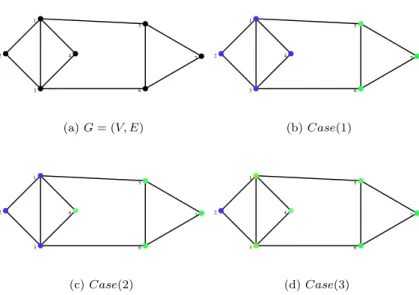
Example 1.2 (Possibility of κ′(G2H)< δ(G) +δ(H).)
The graph G shown in the Figure 2(a) has κ′(G) = 1, δ(G) = 2 and the graph H shown in the Figure 2(b) has κ′(H) = 1, δ(H) = 1. Then δ(G) +δ(H) = 3. The graph G2H shown in the Figure 2(c) hasκ′(G2H) = 2. For this graph, we haveδ(G) +δ(H)> κ′(G2H).
Definition 1.10 (Diameter)
LetG= (V(G), E(G))be a graph. The distance between two verticesvi, vj ∈V(G)of the graphG is denoted bydist(i, j)is the length of a shortest path between vertexvi andvj. Maximum distance between any pair of vertices of the graph is called diameter and denoted bydiam(G).
(a)G (b)H (c)G2H
Figure 2: Edge connectivity for G2H.
Definition 1.11 (Permutation matrix)
Let G = (V(G), E(G)) be a graph. The permutation ϕ defined onV(G) can be represented by a permutation matrixP = (pij), where
pij =
{ 1 ifvi=ϕ(vj), 0 otherwise.
Definition 1.12 (Automorphism)
LetG= (V(G), E(G))be a graph. Then a bijectionϕ:V(G)→V(G)is an automorphism ofGif it preserves the adjacency relation ofG. In other words automorphisms ofGare the permutations of a vertex setV(G)that maps edges onto edges.
Proposition 1.1 (Biggs [6])
LetA(G)be the adjacency matrix of a graphG, andP be the permutation matrix of permutationϕ defined onV(G). Thenϕis an automorphism ofGif and only ifP A=AP.
(Proof ) Let vh = ϕ(vi) and vk = ϕ(vj). Then we have (P A)hj =
∑n l=1
phlalj = aij and (AP)hj =
∑n l=1
ahlplj =ahk. Consequently,AP =P Aif and only ifvi and vj are adjacent, whenever vh andvk are adjacent. That is if and only ifϕis an automorphism ofV(G).
Definition 1.13 (Weighted graph)
A weighted undirected graphG = (V(G), E(G), w), where w is a function from the edge set to the real numbers.
Definition 1.14 (Weighted adjacency matrix) The weighted adjacency matrixW = (wij)is defined as
wij =
{ w(i, j) if(i, j)∈E(G), 0 otherwise.
The degreedi of a vertex vi of a weighted graph is defined by di =
∑n j=1
wij. Unweighted graphs are special cases, where all edge weights are 0 or 1.
Definition 1.15 (Graph cut)
A subset of edges which disconnects the graph is called a graph cut. Let G= (V(G), E(G), w)be a weighted graph and W = (wij)the weighted adjacency matrix. Then for A, B⊂V andA∩B =∅, the graph cut is denoted bycut(A, B) = ∑
i∈A,j∈B
wij.
Definition 1.16 (Isoperimetric number)
The isoperimetric numberi(G)of a graphGof ordern≥2is defined as i(G) = min{cut(S, V \S)
|S| , S⊂V(G),0<|S| ≤ n 2}. Definition 1.17 (Cheeger constant-edge expansion)
LetG= (V(G), E(G))be a graph. For a non empty subsetS⊂V(G), define hG(S) = cut(S, V \S)
min(vol(S), vol(V \S)). Then the Cheeger constant(edge expansion) hG is defined as hG= min
S hG(S).
Definition 1.18 (Cheeger constant-vertex expansion)
LetG= (V(G), E(G))be a graph. For a non empty subsetS⊂V(G), define gG(S) = vol(δS)
min(vol(S), vol(V \S)), where δS = {v /∈ S : (u, v) ∈ E(G), u ∈ S}. Then the Cheeger constant(vertex expansion)gG is defined asgG= min
S gG(S).
Remarks. Here we use notation δS to represent the vertices belong to the set V \S, where each vertex is an endpoint of the edge cut set. This notation is different from theδ(G), which we use to represent the minimum degree of a graph.
Definition 1.19 (Weighted difference Laplacian)
Theweighted difference LaplacianL(G) = (lij)is defined as
lij =
di−wii ifvi=vj,
−wij ifvi andvj are adjacent andvi̸=vj,
0 otherwise.
This can be written asL(G) =D(G)−W(G). For an unweighted graph,L(G) =D(G)−A(G).
Definition 1.20 (Weighted normalized Laplacian)
Theweighted normalized LaplacianL(G) = (ℓij)is defined as
ℓij =
1−wdjjj ifvi=vj,
−√wij
didj ifvi andvj are adjacent andvi̸=vj,
0 otherwise.
Theorem 1.2
LetGbe a graph. ThenL(G) =D−1/2L(G)D−1/2.
(Proof )LetT = (tij)nn,L(G) = (luv)nnand L(G) = (ℓuv)nn. Then define tij=
{ 1
√di vi =vj, 0 otherwise, and
lij =
di ifvi=vj,
−1 (vi, vj)∈E(G), 0 otherwise.
Letmij =
∑n k=1
tik.lkj, where i= 1, . . . , nandj = 1, . . . , n. Ifi≠ kthentik= 0 andmij= 0. Ifi=k thenmij =tii.lij. Now letℓij =
∑n k=1
mik.tkj. Ifk̸=j thentkj= 0. Ifk=j, thenℓij =mij.tjj. Now we can writeℓij as ℓij = (tii.lij).tjj = 1
√di
.lij
√1 dj. Now consider the following cases.
1. Ifi=j thenℓii= 1
√di.lii. 1
√di = 1, 2. if (i, j)∈E(G) thenℓij = 1
√di
.(−1). 1
√dj
= −1
√didj
, 3. Otherwiselij= 0 and ℓij= 0.
By substituting T =D−1/2, we get L(G) = (ℓij) =D−1/2LD−1/2. Further we can deduceL(G) as L(G) =D−1/2LD−1/2=D−1/2(D−W)D−1/2=I−D−1/2W D−1/2.
Definition 1.21 (Signless Laplacian)
Theweighted signless LaplacianSL(G) = (slij)is defined as slij =
di+wii ifvi=vj,
wij ifvi andvj are adjacent andvi ̸=vj,
0 otherwise.
We write this asSL(G) =D+W.
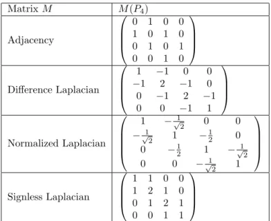
MatrixM M(P4) Adjacency
0 1 0 0 1 0 1 0 0 1 0 1 0 0 1 0
Difference Laplacian
1 −1 0 0
−1 2 −1 0 0 −1 2 −1
0 0 −1 1
Normalized Laplacian
1 −√12 0 0
−√12 1 −12 0 0 −12 1 −√12
0 0 −√12 1
Signless Laplacian
1 1 0 0 1 2 1 0 0 1 2 1 0 0 1 1
Table 1: Matrices associated with graphs.
Example 1.3
The Table 1 shows adjacency matrix and three Laplacian matrices discussed in the above for path graphP4.
Lemma 1.2
LetG= (V(G), E(G), w)be a weighted graph. Then the spectrum ofL(G)andD−1L(G)are equal.
(Proof ) D−1L = D−1(D−W) = I−D−1W = D−1/2DD−1/2−D−1/2D−1/2W = D−1/2(D − W)D−1/2. ThereforeD−1L(G) =L(G) and has the same spectrum.
Lemma 1.3
Let µi(i = 1, . . . , n) be the eigenvalues of difference Laplacian matrix L(G) =D(G)−A(G). Then for any regular graph of degreer, normalized Laplacian eigenvalues areλi=µi
r,(1≤i≤n).
(Proof ) L= (D−A) =rI−A. ThenL(G) =D−1/2LD−1/2 = I
r1/2(rI−A) I
r1/2 =I−A r. Then rL(G) = L(G). If µi is an eigenvalue of L then it is an eigenvalue of rL(G). This implies that λ(L(G)) = µi
r (i= 1, . . . , n).
Proposition 1.2
LetL(G)be the normalized Laplacian matrix of a graphGandP be the permutation matrix corre- sponding to the automorphismϕdefined onV(G). IfU is an eigenvector ofL(G)with an eigenvalue λ, thenP U is also an eigenvector of L(G)with the same eigenvalue.
(Proof ) From the definition of automorphism, PTL(G)P =L(G). Then L(G)U =λU implies that (PTL(G)P)U =λU. SinceP PT =I, we getL(G)P U =λ(P U). IfU is an eigenvector ofL(G)with an eigenvalue λthenP U is also an eigenvector with the same eigenvalue.
Remarks.This result holds for any matrix associated with a graph under the automorphism defined on a vertex set.
Definition 1.22 (Odd-even vectors)
LetG= (V(G), E(G))be a graph andϕ:V →V be an automorphism of order 2. A vectorxis called an even vector ifxi=xϕ(i)for all1≤i≤n and a vectory is called an odd vector ifyi=−yϕ(i) for all1≤i≤n, where n=|V(G)|.
Proposition 1.3
LetGbe a graph,ϕbe an automorphism of Gwith order 2 andP a permutation matrix ofϕ. If an eigenvalue ofL(G)is simple then the corresponding eigenvector is odd or even with respect to ϕ.
(Proof ) Letλbe an eigenvalue,U an eigenvector ofL(G). Ifλis simple thenP U andU are linearly dependent. Then there exists a constantc such thatP U =cU. SinceP2=I for an automorphism of order 2, IU=cP U =c2U andc=±1. ThenP U =U or P U=−U. Hence an eigenvectorU is odd or even with respect to ϕ.
Definition 1.23
LetG= (V(G), E(G))be a graph,|V(G)|=nandU = (u1, u2, . . . , un)an eigenvector ofL(G). We define
V+(U) = {i∈V |ui >0}, V−(U) = {i∈V |ui <0}and
V0(U) = {i∈V |ui = 0}. Lemma 1.4
LetL(G)be the normalized Laplacian of graphGandU = (ui),(i= 1, . . . , n)the second eigenvector.
IfU ̸=0thenV+(U)≠ ∅andV−(U)̸=∅.
(Proof ) The vector D1/2⃗1 is an eigenvector corresponding to the zero eigenvalue. Since the second eigenvector U is orthogonal to D12⃗1, (D12⃗1)TU = 0 and∑
i
√diui = 0. Since di >0, U ̸=0, there exist at least two values such thatui >0 anduj<0 fori̸=j. HenceV+(U)̸=∅ andV−(U)̸=∅. Lemma 1.5
LetGbe a graph with an automorphismϕof order 2. LetU = (u1, u2, . . . , un)be an eigenvector and ϕ(U) = (uϕ(1), uϕ(2), . . . , uϕ(n)). IfU ̸=0andϕ(U) =−U thenV+(U)̸=∅andV−(U)̸=∅.
(Proof ) Assume V+(U) = ∅. If ui ≤ 0,(i = 1, . . . , n), ϕ(U) = −U implies that uϕ(i) > 0. This contradicts that V+(U) =∅. Similarly, if we assume that V−(U) =∅ andui≥0 for(i= 1, . . . , n), then ϕ(U) = −U implies that uϕ(i) < 0. Then this contradicts that V−(U) = ∅. If ui = 0,(i = 1, . . . , n), then U =0and contradicts that U ̸=0.
Proposition 1.4 (Guattery [18])
LetPn be a weighted path graph andL(Pn)be its normalized Laplacian matrix. For any eigenvector X = (x1, x2, . . . , xn)ofL(Pn),
1. x1= 0impliesX= 0, 2. xn= 0impliesX = 0and
3. xi=xi+1= 0implies thatX = 0.
(Proof )
1. We will give the proof by induction. Letn= 2. ThenL(P2)X=λX can be written as ( ℓ11 ℓ12
ℓ21 ℓ22
) ( x1
x2
)
=λ ( x1
x2
) .
Then we have ℓ11x1+ℓ12x2 = λx1 = 0. If x1 = 0 then ℓ12 ̸= 0 implies that x2 = 0, which implies that X = 0. For the induction step, assume that the result holds for L(Pk). Next consider the normalized Laplacian of Pk+1. The first entry of the equation of L(Pk+1)X=λX is,ℓ11x1+ℓ12x2=λx1. Assume thatx1= 0. Thenx2= 0. LetY = (y1, y2, . . . , yk)be the vector containing all entries of X except the first entry x1. Thenx1= 0implies thatx2 =y1= 0. Y is an eigenvector of a normalized Laplacian matrix which obtained by deleting first vertex and edge of Pk+1. That is this represent the L(Pk) and satisfy the equation L(Pk)Y =λY. Since the result holds for allL(Pk) by induction step,x1= 0 implies that Y = 0and hence X= 0.
2. Same arguments implies the result forxn= 0.
3. Assume thatX has two consecutive zerosxi= 0andxi+1= 0. Ifi= 1ori+ 1 =nthenX= 0 by above part 1 and 2 of the proposition. Otherwise, xi+1 = 0implies that first i entries of X are zero by the proof of the part 1 of the proposition. Similarly by a symmetric argument, last n−ientries must also be zero, which gives X = 0.
Lemma 1.6 (Guattery [18])
For a path graphPn,L(Pn)hasnsimple eigenvalues.
(Proof ) Let U = (u1, u2, . . . , un)and U¯ = (¯u1,u¯2, . . . ,u¯n)be the two eigenvectors of L(Pn)with the eigenvalue λ. From the Proposition 1.4, we have un ̸= 0 and u¯n ̸= 0. Let α= u¯n
un
, where α ̸= 0.
Consider L(Pn)(αU−U¯) =λ(αU−U¯). Then-th element of(αU−U¯)is(¯unun−u¯nun) = 0. Then αU = ¯U. Thus U andU¯ are linearly dependent, and henceλis simple.
Proposition 1.5
LetPn = (Vn, En) be a path graph with a vertex setVn ={v1, . . . , vn}. Letϕbe an automorphism of order 2 defined onVn. Then any second eigenvectorU2 ofL(Pn)is an odd-vector.
(Proof ) Let λ2 be the second smallest eigenvalue of L(Pn). Then λ2 > 0 and U2 ⊥ D1/2⃗1. Since λ2 is simple, any eigenvector U2 must be even or odd by the Proposition 1.3. Assume U2 is even.
ThenP U2=U2, whereP is the permutation matrix of an automorphismϕ. From Rayleigh quotient, λ2= min
U2⊥D1/2⃗1
U2TL(G)U2
U2TU2
. Ifnis even, then there exist two center verticesvn
2 andvn
2+1. If(U2)n
2 =
(U2)n
2+1= 0then U2=0by the Proposition 1.4. Hence (U2)n
2 ·(U2)n
2+1̸= 0. Ifnis odd, then there exists a single center vertexv⌈n
2⌉. Ifnis odd andU2 is even then the eigenvector entry corresponding to the center vertex may be zero or non-zero. If this is zero, then we can change the signs of all entries with index less than center vertex and form an odd vector such thatP U2=−U2. Thus it contradicts the simplicity of the eigenvalues. Hence we assume that eigenvector entry corresponding to the center vertex is non zero and its value is c. Now consider the vector X = (−c)⃗1 +U2, where c ̸= 0. Then the eigenvector entry corresponding to the center vertex ofX is zero. Now consider
XTL(G)X
XTX = ((−c)⃗1 +U2)TL(G)((−c)⃗1 +U2) ((−c)⃗1 +U2)T((−c)⃗1 +U2)
= c2.(⃗1TL(G)⃗1) +U2TL(G)U2+ (L(G)U2)T(−c)⃗1 + (−c)⃗1L(G)U2
c2n+U2TU2
= c2.(⃗1TL(G)⃗1) +U2TL(G)U2
c2n+U2TU2
< U2TL(G)U2 U2TU2 .
We can create an odd vector Y, by changing the signs of the eigenvector entries above or below the center vertex, such that YTL(G)YT
YTY = XTL(G)XT
XTX as follows. (Y)i = (X)i, i < n
2 and (Y)i =
−(X)i, i > n
2. Then Y ⊥ D1/2⃗1 and has the same eigenvalue λ2. Since λ2 is simple, we have a contradiction. ThereforeU2 is an odd eigenvector.
Example 1.4 Let
M =
1 −1 0 0 0 0
−1 2 −1 0 0 0
0 −1 2 −1 0 0
0 0 −1 2 −1 0
0 0 0 −1 2 −1
0 0 0 0 −1 1
and
P =
0 0 0 0 0 1
0 0 0 0 1 0
0 0 0 1 0 0
0 0 1 0 0 0
0 1 0 0 0 0
1 0 0 0 0 0
.
If UM is a second eigenvector of M then by Proposition 1.2, P UM is also a second eigenvector.
By Proposition 1.3, P UM = UM or P UM =−UM. By Proposition 1.5, UM is an odd vector and P UM =−UM.
Definition 1.24 (Weighted Path)
LetPn,k = (Pij)be the(n+k)×(n+k)matrix such that Pij =
{ 0 (i=j andi≤n) or (i̸=j+ 1andj̸=i+ 1), 1 (i=j andn+ 1≤i) or (i=j+ 1or j=i+ 1).
Proposition 1.6 Let
P3,4=
0 1 0 0 0 0 0 1 0 1 0 0 0 0 0 1 0 1 0 0 0 0 0 1 1 1 0 0 0 0 0 1 1 1 0 0 0 0 0 1 1 1 0 0 0 0 0 1 1
and
D=
1 0 0 0 0 0 0 0 2 0 0 0 0 0 0 0 2 0 0 0 0 0 0 0 3 0 0 0 0 0 0 0 3 0 0 0 0 0 0 0 3 0 0 0 0 0 0 0 2
.
IfUM be the second eigenvector ofM =D−1/2(D−P3,4)D−1/2thenV+(UM)̸=∅andV−(UM)̸=∅. (Proof ) LetUM be the second eigenvector ofL(M). Then by Lemma 1.4,V+(UM)̸=∅andV−(UM)̸=
∅.
Definition 1.25 (Spectral radius)
Letλ1, λ2, . . . , λn be the (real or complex) eigenvalues of a matrix A. Then the spectral radiusρ(A) is defined asρ(A) = max
i (|λi|),(i= 1, . . . , n).
Definition 1.26 (Positive-definite)
A symmetric matrix Ais called positive-definite, if for all nonzero vectors x∈ ℜn the associated quadratic form given byA(x) =xTAxtakes only positive values.
Definition 1.27 (Semidefinite)
If the quadratic formA(x) =xTAx takes only non-negative values, then the symmetric matrixA is calledpositive-semidefinite.
Definition 1.28 (Indefinite)
The matrix is indefinite, when it is neither positive-semidefinite nor negative-semidefinite.
Definition 1.29 (Girth)
The girth of a graph is the length of a shortest cycle contained in the graph. If the graph does not contain any cycles (acyclic graph), then the girth is defined to be infinity.
1.3 Formal notations for graphs
Let Σ is an alphabet and Σ∗ is a set of strings over Σ including the empty stringϵ. We denote the length of w∈Σ∗ by |w|. Let Σ≤n ={w∈ Σ∗||w|< n} and Σ≤1n ={w∈Σ∗|1 ≤ |w| < n}. In this paper, we assumeΣ ={0,1}.
Definition 1.30 (Complete binary tree)
A complete binary treeTn= (V, E)of depthnis defined as follows.
V = Σ≤n, E = E1∪E2,
E1 = {(ϵ, w)|w∈Σ1≤n,|w|= 1},
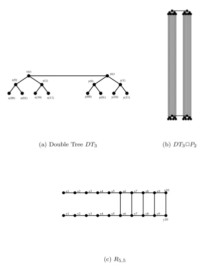
E2 = {(w, wu)|w, u∈Σ≤1n,|wu|< n,|wu|=|w|+ 1}. Definition 1.31 (Double tree)
A double treeDTn = (V, E), wherenis the depth of the tree, consists of two complete binary trees connected by their root. We define double tree as follows.
V = {x(w)|w∈Σ≤n} ∪ {y(w)|w∈Σ≤n},
E1 = {(x(w), x(wu))|w, u∈Σ≤1n,|wu|< n,|wu|=|w|+ 1}, E2 = {(y(w), y(wu))|w, u∈Σ≤1n,|wu|< n,|wu|=|w|+ 1}, E3 = (x(ϵ), y(ϵ)),
E4 = {(x(ϵ), x(w))|w∈Σ1≤n,|w|= 1}, E5 = {(y(ϵ), y(w))|w∈Σ1≤n,|w|= 1},
E =
∪5 i=1
Ei.
Definition 1.32 (Cycle)
A cycle Cn = (Vn, En) consists of a vertex set Vn = {vl | l ∈ Z+, l ≤ n} and an edge set En = {(vl, vl+1)|1≤l < n} ∪ {(v1, vn)}.
Definition 1.33 (Path)
A path Pn = (Vn, En) consists of a vertex set Vn = {vl | l ∈ Z+, l ≤ n} and an edge set En = {(vl, vl+1)|1≤l < n}.
Definition 1.34 (Regular graph)
A graphG= (V(G), E(G))is called r-regular, if degree of each vertex isr.
Definition 1.35 (Complete graph)
A complete graph Kn = (Vn, En) consists of a vertex set Vn = {vi | 1 ≤ i ≤ n} and an edge set En={(vi, vj)|i̸=j and1≤i≤n,1≤j≤n}.