Evaluation of Various Cache Extensions for LSTM Based Language Models

全文

(1)Vol.2017-NL-231 No.5 Vol.2017-SLP-116 No.5 2017/5/15. IPSJ SIG Technical Report. Evaluation of Various Cache Extensions for LSTM Based Language Models Hentschel Michael1,2,a). Ogawa Atsunori2,b). Delcroix Marc2,c). Nakatani Tomohiro2,d). Abstract: Memory in recurrent neural networks is currently an issue. There have been various successful projects in recent years which enlarged the memory of neural networks. When applied to language modelling, these techniques showed a significant reduction in perplexity. However, on the downside these models are very costly to train as they have many parameters and are very complex. Therefore recently, simpler models were presented, which do not suffer from this drawback. The extensions to long short-term memory language models we present in this paper draw ideas from the cache model for N-gram language models from the early 90s. We evaluate all models in terms of perplexity and word error rate on the MIT-OCW lecture corpus. Keywords: Language Model, Neural Network, LSTM, RNN, Cache. 1.. Introduction. The current state-of-the-art in language models (LM) has been dominated by neural network based language models for a few years. The first to propose the application of neural networks to lanugage modelling were Bengio et al. in 2003 [1], when they introduced feed forward neural networks to LMs. Later, Mikolov et al. presented LMs based on recurrent neural networks (RNN) [2] because these models have a better ability to capture long term dependencies. However, RNNs suffer from various problems like exploding and vanishing gradients [3], so Sundermeyer et al. proposed using long short-term memory (LSTM) [4] based networks [5]. However, recent research suggests, that these kinds of neural networks do not have sufficient memory. This was first demonstrated by neural touring machines [6] which showed more effective to abstract beyond the training data compared to LSTMs. In one of the tasks, the network had to learn a simple sequence copy algorithm and it showed to be successful in learning this copy algorithm and abstracting to sequences of arbitrary length. Memory networks [7][8], which share a similar idea were able to outperform simpler RNN or LSTM models on a question answering task and on perplexity evaluation on the Penn Treebank dataset [9]. Using this idea, the authors in [10] proposed recurrent memory networks, which combine an LSTM and the memory cell from the memory network. They evaluated their model in terms of perplexity on datasets for three languages and a sentence 1. 2. a) b) c) d). Nara Institute of Science and Technology, 8916-5 Takayama, Ikoma, Nara, Japan NTT Communication Science Laboratories, NTT Corporation, 2-4, Hikaridai, Seika-cho, Kyoto, Japan [email protected] [email protected] [email protected] [email protected]. c 2017 Information Processing Society of Japan. completion task. Furthermore, stack-augmented recurrent neural networks [11], i.e., a recurrent network which has the ability to read from and write to a stack, were investigated on the task of learning simple algorithmic patterns. The problem with the above models is, however, that they are time consuming to train because the network has to learn the memory access mechanism. This mechanism is in many cases implemented by calculating attention vectors on the memory and the input to the network. A simpler way to extend neural networks with memory has recently shown to be very effective in the context of language modelling. First, a pointer network [12] based approach [13] and second a neural cache based approach [14]. In the former one, the pointers enable the network to establish direct connections from the input to the output and in this way make use of out-of-vocabulary (OOV) words on the input in the network’s prediction. In the latter one, the hidden state of the network and the true output label is used to calculate a probability from the cache for the next word. In terms of language modelling, there have been other approaches in recent years based on the classic concept of bag-ofwords (BOW). In order to make use of the information in preceding dialog turns, the authors in [15] extended a feed forward neural network with a cache component that captures information about previous turns. RNNs extended with a BOW cache were introduced by [16] and [17]. The BOW input was an exponentially decaying cache for the whole history. The authors of all aforementioned papers applied their respective models to various tasks, not limited but including natural language processing. However, our main interest is speech recognition and in particular the effectiveness of LMs in n-best rescoring. Therefore, in this paper we compare several cache extensions based on the afore mentioned ones. First, we investigate the effectiveness of the continuous neural cache from [14] and in addition a direct combination of this cache with an LSTM based LM. Sec-. 1.

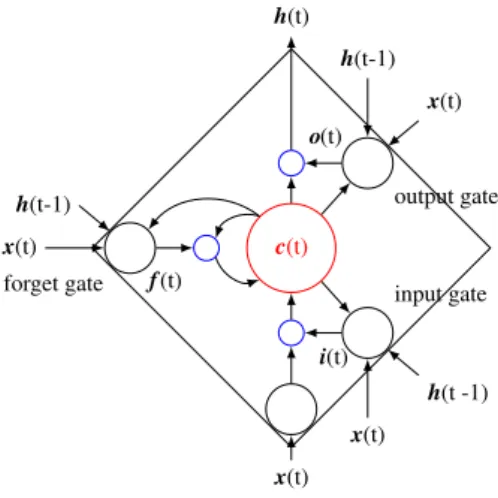
(2) Vol.2017-NL-231 No.5 Vol.2017-SLP-116 No.5 2017/5/15. IPSJ SIG Technical Report. (h(t − 1), w(t)). h(t). (h(t − 2), w(t − 1)). h(t-1). (h(t − 3), w(t − 2)). x(t). w(t ˆ + 1) V. o(t) h(t-1) x(t) forget gate. output gate. h(t − 3). input gate. w(t − 3). c(t). h(t − 2). U. f (t). h(t − 1). U. h(t). U. w(t − 2). U. w(t − 1). w(t). Fig. 2 Continuous neural cache model as proposed by [14].. i(t) h(t -1). (h(t − 1), w(t)). x(t). (h(t − 2), w(t − 1)). x(t). hc (t). (h(t − 3), w(t − 2)). Fig. 1 An LSTM cell. cache. c(t). Vc. Uc. ond, we analyse an extension to an LSTM that is inspired by the BOW cache from [16] and [17]. We provide perplexity (PPL) and word error rate (WER) results on an MIT lecture corpus [18]. The results and findings we present in this paper can be seen as a current status of ongoing research.. 2.. i(t) = σ(W i,w x(t) + W i,h h(t − 1) + bi ). (1). f (t) = σ(W f,w x(t) + W f,h h(t − 1) + b f ). (2). o(t) = σ(W o,w x(t) + W o,h h(t − 1) + bo ). (3). g(t) = tanh(W g,w x(t) + W g,h h(t − 1) + bg ). (4). c(t) = f (t)

(3) c(t − 1) + i(t)

(4) g(t). (5). h(t) = o(t)

(5) tanh(c(t)). (6). i, f and o are usually named the input, forget and output gate, respectively. W y,w and W y,h denote the weight matrices for gate y for the word input and the previous hidden layer, respectively. biasy are the bias vectors for the respective gates. Since we use vector notation in the above equations, σ(·) is the element wise sigmoid, tanh(·) is the element wise hyperbolic tangent and

(6) denotes an element wise multiplication. We denote the time index t in brackets after the corresponding vector.. Continuous Neural Cache. 3.1 External Cache An effective way to implement a continuous neural cache (NC) was presented in [14]. In this method, the cache consists of a list of tuples (h(t), w(t + 1)), where h(t) is the hidden state of the network at time t and w(t + 1) the target label the network should predict at step t. The input word vector w(t) to the network is encoded as a one-hot vector and the input to the LSTM is obtained by multiplication with a linear layer U. The cache is shown with an unfolded structure in Fig. 2. The probability for each possible element i in the output vector w(t ˆ + 1) is calculated from the cache as follows.. c 2017 Information Processing Society of Japan. +. LSTM U. w(t ˆ + 1). V. Fig. 3 Continuous connected neural cache to the softmax of an LSTMLM.. pcache (w(t ˆ + 1)(i) |cache) ∝ N X. T (i) =w (t−n+1)(i) exp(θh(t) hc (t − n). 1w(t+1) ˆ c. LSTM. A single LSTM cell is shown in Fig. 1. In the language model multiple of these cells are used and they are described by the following set of equations.. 3.. w(t). (7). n=1. The elements of the cache are denoted by a subscript c to distinguish them from the current state of the network. 1a=b is a function that evaluates to one if a is equal to b and is zero for all other cases. θ is a positive real valued parameter. N is the size of the cache, which makes the cache cover all the current history ranging from the last time step t − 1 to t − N. On can interpret this function as a similarity measure for the history stored in the cache and the current hidden state. By multiplying this similarity with 1a=b it is restricted only to the cases, where the previous target of the network matches the i-th word in the output. In order to obtain a probability from the cache, we sum over all elements in the resulting vector, i.e., summing over the vocabulary size, and divide all entries by this sum. That means we normalise the cache output that all elements in the vector sum up to one. A major advantage of this cache, as stated by the authors in [14], is the fact that the network does not need to be trained together with the cache. The output of the cache is simply linearly interpolated with the output of the network and does not influence the parameters of the network. Therefore, there is no training time increase. 3.2 Connected Neural Cache Taking the idea from Section 3.1 and Section 4, we connected the continuous neural cache to the network directly. Fig. 3 shows the cache connected to the softmax output layer. By integrating the cache directly into the network and performing a joint optimisation of the parameters, the network should be able to learn a better combination weights for each individual word. Through the linear layers, we can use an individual interpolation weight for each word, depending on the context. The input to the LSTM can thus be formulated as 2.

(7) Vol.2017-NL-231 No.5 Vol.2017-SLP-116 No.5 2017/5/15. IPSJ SIG Technical Report. hu (t) cu (t) . . .. hb (t). Uu. cb (t). unigram. bigram Vb. Ub w(t). +. LSTM U. Vu y(t). w(t ˆ + 1). V. Fig. 4 BOW extension for an LSTMLM.. x(t) = Uw(t) + Uc hc (t). (8). with hc begin the output of the hidden layer after the cache. The input to the softmax can be written as y(t) = Vh(t) + V c hc (t).. (9). Since the cache is computationally expensive, we combine the cache with a pre-trained base model and only train the weights in the linear layers for the cache. The parameters of the base model are left unchanged except for the linear layer before the softmax V. As a modification to the original cache implementation, we also investigate a cosine word similarity measure instead of a hard word identity. Using a similarity measure, also words which are similar (in the vector space) to word i will be assigned some probability mass. We expect similar words to appear in a semantically similar context (e.g. ’cat’ and ’dog’).. 4.. Bag-of-Words Cache. A simple form of a cache extension is BOW. In [16] and [17] the authors used an exponentially weighted BOW cache. An exponentially decaying weight is multiplied with all words up to the current time t, where the latest word has the highest weight and the word seen first the lowest weight. Afterwards these weighted word vectors are summed up and put into the network. Our approach is similar, but we do not keep a continuously updated BOW. We use a cache of N entries and each entry in the cache gets an exponentially decaying weight, where the word first in the cache has the highest and the word occurring last has the lowest weight. cu (t) =. PN−1 n=0. w(n) exp(−n),. (10). where w(n) is the n-th vector in the cache. The cache itself can be thought of as an ordered list. The elements in the list (i.e. the words) are sorted according to their order of appearance. However, each word is only contained once in the list. If a new word appears, the last word in the list, i.e., the word appearing least frequently in the recent past, is removed from the cache and the new word is inserted at the head of the list. If a word re-appears, it is taken from its current position and inserted at the head of the list. We call this cache the unigram cache, as it contains the information about the last most frequent N unigrams in the recent past. This cache is highlighted in red in Fig. 4. Since many words appearing frequently in the corpus (e.g.. c 2017 Information Processing Society of Japan. ’the’ or ’a’) don’t carry important information, we exclude frequent words from the cache. The frequency is estimated on the training data. Likewise, words appearing infrequently in the training data are unlikely to appear often in the evaluation data. Therefore, we also exclude infrequent words from the cache, where we again estimate the frequency on the training data. In addition to this unigram cache, we also use a bigram cache. One can think of the bigram cache as another list attached to each unigram. That means, for each unigram there exist a list with the last M words appearing after this unigram. Again the same ordering and insertion policy as with unigrams is used, i.e., the word appearing most recently is at the head of the list. However, we do not use the threshold on the frequency for the bigram cache. The bigram cache is highlighted in blue in Fig. 4. The calculation for cb (t) is the analogue to the calculation of cu (t) in Equation 10. Fig. 4 shows the final model. The output of both caches is a vector of equal length as the vocabulary size. These vectors are compressed by a linear layer with a subsequent non-linearity (reLU in our case). The dimension if the hidden layer is chosen to be equal to the number of LSTM units. We introduce this reduction for two reasons. First, it acts a a non-linear dimension reduction and second, it speeds up the computation because the number of parameters is significantly reduced. The output of the hidden layer is combined with the output of the LSTM before the softmax. The Input to the LSTM can then be written as h(t) = Uw(t) + Uu hu (t) + Ub hb (t),. (11). with hu and hb being the outputs of the hidden layer for the unigram and bigram cache respectively. The input to the softmax can be written as y(t) = Vh(t) + V u hu (t) + V b hb (t).. (12). The direct connection of the cache output to the output layer, i.e., the softmax, is inspired by several prior research. [17] proposed direct a connection in the case of using an RNN instead of an LSTM. To a further extend it is also related to the idea of highway networks [19] and residual connections [20] which have proven useful when training deeper networks.. 5.. Experiments. 5.1 Setup For our experiments we performed PPL evaluation and N-best rescoring on the MIT-OCW lecture corpus [18]. The corpus has about 6M words and the vocabulary size is 47K. We did not truncate the vocabulary. The corpus has about 100h of transcribed speech. As speech recogniser, we used a GMM-HMM based system as also used in [21]. This speech recogniser achieved a WER of 26.7% without rescoring. Our LSTM LM implementation used the deep learning toolkit chainer [22]. We trained all LMs with mini-batches of length 128 and did truncated backpropagation through time for 20 words. The initial learning rate was set to 0.1 and decreased by a factor of 1.3 after the sixth epoch. As optimiser we used AdaGrad [23] and all models were trained for 16 epochs. For training we also used dropout. 3.

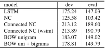
(8) Vol.2017-NL-231 No.5 Vol.2017-SLP-116 No.5 2017/5/15. IPSJ SIG Technical Report. Table 1 PPL results for development and evaluation data of MIT-OCW. model LSTM NC Connected NC Connected NC (wsim) BOW unigram BOW uni + bigrams. dev 175.24 125.58 213.12 213.89 183.07 178.81. eval 147.03 103.42 189.60 190.79 149.02 149.79. Table 2 WER results for 100-best rescoring on MIT-OCW. model LSTM NC Connected NC Connected NC (wsim) BOW unigram BOW uni + bigram. WER 24.3 24.2 25.2 25.3 31.5 31.7. For the networks with the neural connected cache, we connected the neural cache to an LSTM model which was trained for 16 epochs. In the training we only re-trained the connections in the linear layer before the softmax of the base LSTM and the linear layers of the cache for 5 epochs with a LR of 0.1. The LR decreased by 1.3 every epoch. To calculate the word error rate in N-best rescoring, we interpolated the LSTM log probability with a trigram probability and the acoustic model score. The trigram LM was trained using the SRILM toolkit [24] and used Kneser-Ney [25] smoothing. The trigram itself gave a PPL of 199 on the evaluation data. 5.2 PPL Evaluation At first we investigated the PPL of different models as shown in Table 1 on the development and evaluation data. The baseline trigram gave a PPL of 199. Our Chainer LSTM baseline gave a PPL of 147.03. Using the continuous cache from Section 3.1, we achieved an improvement of roughly 30% on the evaluation data to 103.42. This result corresponds to the numbers reported in [14]. However, connecting the cache directly to the softmax layer did not give any improvement. Interestingly, the PPL remained more or less constant during training, which means that the network did not learn good parameters for the interpolation with the cache. Also, using a word similarity (wsim) measure instead of the probability for the word vector did not change the result. For the BOW cache we investigated two scenarios. In the first case, we only used the unigram information hu (t) and in the second we sued both unigram hu (t) and bigram hb (t) information. In both cases the PPL raised slightly compared to the LSTM only baseline. 5.3 ASR Experiments Table 2 shows the results for n-best rescoring on the 100-best list we obtained with SOLON speech recogniser [26]. Without rescoring, the speech recogniser achieved a WER of 26.7%. For the baseline system in 100-best rescoring with an LSTM we obtained a WER of 24.3%. With the continuous cache, although the PPL reduction was significantly high, the WER only improved by 0.1% (absolute) over the LSTM. One possible explanation for this result is, that. c 2017 Information Processing Society of Japan. during PPL evaluation the cache can be filled with the true nextword information. In rescoring however, we can only access hypothesises. In addition, a hypothesis with multiple word insertions and replacements might get a higher score than a single utterance with just one word substitution, because the former one is more likely from the LM’s perspective. Further reasons are that the cache outputs probability zero in many cases and the capability of the cache to predict OOVs is irrelevant for rescoring. As expected from the PPL results, the neural connected continous cache did not achieve any improvements in WER over the baseline. Using the BOW cache, the WER increased dramatically. The results were even worse than those after the first pass only. Such a behaviour was no expected from the PPL evaluation where performance dropped a little bit. So far we do not have any good explanation why the WER increased so dramatically.. 6.. Conclusion. We evaluated two conceptually different cache extensions, i.e., continuous neural cache and BOW, connected to LSTMs. However, in our experiments the effect of the cache on the LSTM was the opposite from what we anticipated. The continuous neural cache was successful in reducing the PPL but overall we did not observe a significant benefit during n-best rescoring. With the BOW cache, however, although PPL evaluation was only slightly worse compared to the baseline, during rescoring the cache severely decreased performance. Overall, we conclude that the cache implementations we investigated were not effective for our dataset on the task of rescoring in ASR. References [1] [2] [3] [4] [5] [6] [7] [8] [9] [10] [11] [12] [13] [14]. Bengio, Y., Ducharme, R., Vincent, P. and Jauvin, C.: A neural probabilistic language model, Journal of machine learning research, Vol. 3, No. Feb, pp. 1137–1155 (2003). Mikolov, T., Karafiát, M., Burget, L., Cernock`y, J. and Khudanpur, S.: Recurrent neural network based language model., INTERSPEECH, Vol. 2, pp. 1045–1048 (2010). Bengio, Y., Simard, P. and Frasconi, P.: Learning long-term dependencies with gradient descent is difficult, IEEE transactions on neural networks, Vol. 5, No. 2, pp. 157–166 (1994). Hochreiter, S. and Schmidhuber, J.: Long short-term memory, Neural computation, Vol. 9, No. 8, pp. 1735–1780 (1997). Sundermeyer, M., Schlüter, R. and Ney, H.: LSTM Neural Networks for Language Modeling., INTERSPEECH, pp. 194–197 (2012). Graves, A., Wayne, G. and Danihelka, I.: Neural turing machines, arXiv preprint arXiv:1410.5401 (2014). Weston, J., Chopra, S. and Bordes, A.: Memory networks, arXiv preprint arXiv:1410.3916 (2014). Sukhbaatar, S., Weston, J., Fergus, R. et al.: End-to-end memory networks, Advances in neural information processing systems, pp. 2440– 2448 (2015). Marcus, M. P., Marcinkiewicz, M. A. and Santorini, B.: Building a large annotated corpus of English: The Penn Treebank, Computational linguistics, Vol. 19, No. 2, pp. 313–330 (1993). Tran, K., Bisazza, A. and Monz, C.: Recurrent memory networks for language modeling, arXiv preprint arXiv:1601.01272 (2016). Joulin, A. and Mikolov, T.: Inferring algorithmic patterns with stackaugmented recurrent nets, Advances in neural information processing systems, pp. 190–198 (2015). Vinyals, O., Fortunato, M. and Jaitly, N.: Pointer networks, NIPS, pp. 2692–2700 (2015). Merity, S., Xiong, C., Bradbury, J. and Socher, R.: Pointer Sentinel Mixture Models, arXiv preprint arXiv:1609.07843 (2016). Grave, E., Joulin, A. and Usunier, N.: Improving Neural Language Models with a Continuous Cache, arXiv preprint arXiv:1612.04426 (2016).. 4.

(9) IPSJ SIG Technical Report. [15]. [16] [17]. [18] [19] [20] [21]. [22]. [23] [24] [25] [26]. Vol.2017-NL-231 No.5 Vol.2017-SLP-116 No.5 2017/5/15. Zamora-Mart´ınez, F., Espana-Boquera, S., Castro-Bleda, M. and DeMori, R.: Cache neural network language models based on longdistance dependencies for a spoken dialog system, 2012 IEEE International Conference on Acoustics, Speech and Signal Processing (ICASSP), IEEE, pp. 4993–4996 (2012). Irie, K., Schlüter, R. and Ney, H.: Bag-of-words input for long history representation in neural network-based language models for speech recognition, INTERSPEECH, pp. 2371–2375 (2015). Haidar, M. A. and Kurimo, M.: Recurrent Neural Network Language Model With Incremental Updated Context Information Generated Using Bag-of-Words Representation, Interspeech 2016, pp. 3504–3508 (2016). Glass, J., Hazen, T. J., Cyphers, S., Malioutov, I., Huynh, D. and Barzilay, R.: Recent progress in the MIT spoken lecture processing project, INTERSPEECH, pp. 2553–2556 (2007). Srivastava, R. K., Greff, K. and Schmidhuber, J.: Highway networks, arXiv preprint arXiv:1505.00387 (2015). He, K., Zhang, X., Ren, S. and Sun, J.: Deep residual learning for image recognition, IEEE Conference on Computer Vision and Pattern Recognition, pp. 770–778 (2016). Hori, T., Kubo, Y. and Nakamura, A.: Real-time one-pass decoding with recurrent neural network language model for speech recognition, 2014 IEEE International Conference on Acoustics, Speech and Signal Processing (ICASSP), IEEE, pp. 6364–6368 (2014). Tokui, S., Oono, K., Hido, S. and Clayton, J.: Chainer: a NextGeneration Open Source Framework for Deep Learning, Proceedings of Workshop on Machine Learning Systems (LearningSys) in the Twenty-ninth Anual Conference on Neural Information Processing (NIPS) (2015). Duchi, J., Hazan, E. and Singer, Y.: Adative subgradient methods for online learning and stochastic optimization, Journal of Machine Learning Research, Vol. 12, No. Jul, pp. 2121–2159 (2011). Stolcke, A.: SRILM – an extensible language modeling toolkit, International Conference on Speech and Language Processing, pp. 901– 904 (2002). Kneser, R. and Ney, H.: Improved backing-off for m-gram language modeling, 1995 IEEE International Conference on Acoustics, Speech, and Signal Processing (ICASSP), Vol. 1, IEEE, pp. 181–184 (1995). Hori, T.: NTT Speech recognizer with OutLook On the Next generation: SOLON, Proc. NTT Workshop on Communication Scene Analysis, 2004 (2004).. c 2017 Information Processing Society of Japan. 5.

(10)