Spatial and temporal variations of river
metabolism along a latitudinal gradient across
Japan.
著者
GURUNG ANANDEETA
学位授与機関
Tohoku University
学位授与番号
11301甲第18950号
Doctoral Thesis
Spatial and temporal dynamics of river metabolism along
a latitudinal gradient
Gurung Anandeeta
Graduate School of Life Sciences
Tohoku University
Table of Contents
Chapter 1 General Summary 1
Chapter 2 River metabolism along a latitudinal gradient across Japan and in a global scale
6
Chapter 3 Latitudinal comparisons of river metabolism reveal larger seasonal variations toward north
46
Chapter 4 Effects of land use and land cover on a latitudinal gradient of river metabolism in Japan
104
Acknowledgements 139
Chapter 1
River metabolism is the balance between carbon fixation through gross primary production (GPP) and mineralization of autochthonous and allochthonous organic matter through ecosystem respiration (ER). A river is autotrophic if production is higher than respiration, and heterotrophic if respiration is higher than production. Generally, river ecosystems tend to be heterotrophic since in addition to autochthonous organic carbon fixed by autotrophs within rivers, allochthonous organic carbon is also discharged from terrestrial ecosystems into rivers and respired. Therefore, measurement of river metabolic rates (i.e. GPP and ER rate) are of prime importance in determining and evaluating the ecological state of rivers. River metabolic rates can be measured by diel changes in dissolved oxygen (DO) concentrations which is determined by the balance between instantaneous production and respiration rates in rivers and gas flux between river water and air known as reaeration rate (K).
Classically, it has been expressed as: ∆𝐷𝑂
𝑑𝑡 = 𝐺𝑃𝑃 − 𝐸𝑅 + 𝐾
where ∆𝐷𝑂 is difference in DO concentration for a short time interval. Therefore, if temporal estimations of DO and reaeration rates are available, both GPP and ER rates can be empirically estimated. Due to the development of DO measurement probes, it has become possible to automatically measure high frequency in situ DO concentrations. However, since estimation of reaeration rate was experimentally laborious and imprecise, it has been difficult to estimate the GPP and ER rates from this type of equation. Fortunately, recent progress in mathematical models with Bayesian algorithms, such as BASE v2.0 model (Grace et al. 2015), have made it possible to determine reaeration rates simultaneously with estimations of GPP and ER rates.
In Japan, the Ministry of Land, Infrastructure, Transport and Tourism (MLIT) has routinely measured diurnal changes in DO and water temperature at monitoring sites of the major rivers and provides these data as an open access database named Water Information System. Using these
measured DO values with a modern statistical modelling, I estimated GPP, ER and NEP rates in various rivers of the Japanese Archipelago.
In the next chapter, I examined if river metabolic rate changes spatially along latitude. Since temperature is a key factor affecting photosynthetic and respiration rates, the rates of GPP and ER are expected to be lower for rivers at higher latitudes, while the NEP rate likely decrease in rivers at lower latitude due to higher sensitivity of ER to temperature compared with GPP. To examine these possibilities, I estimated the ecosystem metabolism of 30 rivers located from 43.037°N to 32.386°N in Japan during summer using a Bayesian model with hourly changes in dissolved oxygen concentrations. In addition, I examined latitudinal trends of GPP, ER and NEP in a global scale by compiling and analyzing river metabolic data estimated in previous studies. This analysis showed that both GPP and ER tended to increase with latitude, although these rates were positively related to water temperature in Japanese rivers. Global dataset of GPP and ER also showed increasing trend towards higher latitude. In addition, contrary to my initial expectations, NEP decreased with latitude and most rivers were net heterotrophic at both regional (Japanese rivers) and global scales. These results imply that the latitudinal temperature effect on river metabolism is masked by other factors not examined in this study, such as land use in the watershed, which play pivotal roles in explaining the latitudinal variation of river metabolism.
In the following chapter, I estimated river metabolic rates in four seasons from 2010 – 2016 at 16 river stations across Japan to examine magnitude of annual and seasonal variations in river GPP and ER rates and if these variations change across the latitudinal gradient. The analyses showed that seasonal variation across the rivers was greater than annual variations in the GPP rates, while, the annual variations in ER rates was often higher than, or the same level to, the seasonal variations, indicating that seasonality is stable in the GPP rate than in the ER rate in river ecosystems. Temperature, precipitation and photosynthetically active radiation (PAR) explained
50% of the seasonal variation in the GPP rate while temperature, precipitation and GPP rate explained 27% of the seasonal variation in ER rate. More importantly, I found that magnitudes of seasonal variabilities in the GPP and ER rates tended to increase toward north. Although, the magnitude of seasonal variability along the latitude gradient in the ER rates was well explained by temperature and GPP rate, seasonal variability along the latitudinal gradient in the GPP rates were not explained by temperature and PAR, suggesting that seasonal and spatial responses of the river GPP rate to changes in environmental conditions differ with those of ER rate, and that the magnitude of seasonal variability in GPP is determined by local environmental conditions independent of the latitudinal environmental trend.
In the last chapter, I examined the hypothesis that land use and land cover in the watershed play a pivotal role in explaining the latitudinal variation of river metabolic rates. For this objective, I examined land use and land cover in the watersheds of 23 Japanese rivers across the latitudinal gradient of 43.037°N to 32.386°N at eight different spatial scales. The analysis showed that land use and land cover components have different effects on metabolic rates depending on the distance from the location where these rates were measured. For example, GPP rate was affected by near-distance agriculture and forest areas and far-near-distance agriculture and grassland areas and ER rate was affected by near-distance agriculture and urban areas and far-distance grassland areas. More importantly, the results supported the hypotheses that increasing trends of GPP and ER rates toward north rivers were indeed generated by latitudinal differences in land use and land covers in the watershed. Latitudinal variations in the river metabolic rates suggests that the balance of GPP and ER rates in given river ecosystem will change under putative warming. However, this study suggests that changes in land use and land cover induced by anthropogenic activities in the watersheds would have greater impacts on the balance between the GPP and ER rates in given river ecosystems.
References
1. Grace, M. R., D. P. Giling, S. Hladyz, V. Caron, R. M. Thompson, and R. Mac Nally. 2015. Fast processing of diel oxygen curves: Estimating stream metabolism with base (BAyesian single-station estimation). Limnol. Oceanogr. Methods 13: 103–114. doi:10.1002/lom.10011
Chapter 2
Introduction
Ecosystem metabolism includes carbon fixation and mineralization through gross primary production (GPP) and ecosystem respiration (ER). In rivers, the balance between GPP and ER, denoted by net ecosystem production (NEP), is not necessarily positive since, in addition to organic carbon fixed by autotrophs within rivers, terrigenous organic carbon is discharged into rivers and respired (Marcarelli et al. 2011; Hotchkiss et al. 2015). This implies that river communities are sustained by both autochthonous and allochthonous organic carbon and that the community dependency on the terrigenous carbon is reflected by the balance of fixation and mineralization of organic carbon. Thus, GPP, ER and NEP are important properties integrating the biological processes of communities involved and characterizing given river ecosystems (Mulholland et al. 2001; Hotchkiss et al. 2015).
River metabolism is known to be influenced by various abiotic and biotic factors such as light (Naiman 1983; Bott et al. 1985; Mulholland et al. 2001; Roberts et al. 2007; Finlay 2011; Beaulieu et al. 2013), temperature (Demars et al. 2011; Beaulieu et al. 2013; Escoffier et al. 2016), nutrients (Acuña et al. 2007; Iwata et al. 2013; Masese et al. 2017), hydromorphology (Young et al. 2008; Kupilas et al. 2017), geomorphology (Uehlinger 2006; Atkinson et al. 2008), and changes spatially and seasonally. Among these, previous studies have shown that GPP is affected mainly by light (Naiman 1983; Bott et al. 1985; Mulholland et al. 2001; Roberts et al. 2007; Finlay 2011; Beaulieu et al. 2013) and temperature (Demars et al. 2011; Beaulieu et al. 2013; Escoffier et al. 2016), while ER is controlled mainly by temperature (Bott et al. 1985; Webster et al. 1995; Acuña et al. 2004; Uehlinger 2006; Demars et al. 2011). In addition, some studies suggested that ER is more responsive to temperature compared with GPP (Allen et al. 2005; Song et al. 2018). Thus, GPP, ER and NEP in rivers may systematically change with the latitudinal gradient of light and temperature. If this were the case, the latitudinal gradient would be useful to build predictive models of river ecosystem metabolism in response to warming and climate changes. However,
although a few studies have examined the latitudinal variations of GPP (Lamberti and Steinman 1997) in rivers, no study has yet examined latitudinal variations of ER and thus NEP.
In this study, therefore, I simultaneously estimated GPP, ER and NEP in rivers at various latitudes in Japan. Since Japan extends over a wide range of latitudes from 24°N to 45°N, it provides an excellent location to examine these hypotheses. In Japan, the Ministry of Land, Infrastructure, Transport and Tourism (MLIT) has routinely measured diurnal changes in DO and water temperature at monitoring sites of major rivers and provides these data as an open access database (Water Information System, http://www1.river.go.jp). Using these measured DO values with a modern statistical modelling, I estimated GPP, ER and NEP in various rivers of Japan. Then, I examined the following hypotheses: (1) GPP would decrease towards the north since both temperature and the amount of solar radiation decrease from lower to higher latitudes, (2) ER would also be lower in areas of higher latitude since lower temperatures reduce the respiration activity of organisms; and accordingly, (3) river ecosystems would become more heterotrophic in rivers located at lower latitude since ER is more sensitive to changes in temperature than GPP (Allen et al. 2005; Song et al. 2018). Finally, to test if the latitudinal trends of GPP, ER and NEP found in Japan rivers are valid in a spatially larger scale, I complied and examined literature data on GPP and ER estimated in rivers at various latitude in the world and compared the latitudinal trends with those in Japanese rivers.
Materials and Methods
Study area
The Japanese Archipelago (area: 377,880 km2) extends over approximately 2,000 km from
subtropical in the south to subarctic climatic conditions in the north (Iyama 1993; Yoshimura et al. 2005) and has four distinct seasons (Japan Meteorological Agency 2016). In general, summer
extends from mid-June to September, with early summer experiencing a rainy season, known as the Tsuyu. During the late summer and autumn, typhoons strike the archipelago, which often result in heavy rains and river flooding. In the northern areas, snowfall occurs during the winter, when river flow is generally low. In such snow-covered areas, river flow becomes high during the spring with snowmelt runoff. As a result, river flow fluctuates seasonally and annually depending on the rainfall and snowmelt patterns (Yanai 2008). Geologically, Japan is characterized by frequent tectonic and geothermal activity. Japanese rivers are generally short (max length: 370 km) and steep, with flashy flow regimes and thus are sediment rich (Yoshimura et al. 2005).
In this study, I focused on the metabolic rates in August since it falls before the typhoon season and after the early summer rainy season, and thus the weather conditions are relatively stable throughout the country. In addition, the high temperatures in this month cause high biological activity, which likely intensifies the latitudinal gradients.
Data collection
I collected river data in August from the database constructed by the Water Information System (WIS: http://www1.river.go.jp/) developed by MLIT, except for Mimi River (ID = 30, Table 1), which was provided by the Central Research Institute of Electric Power Industry (CRIEPI). The WIS database provides water level, discharge, DO, pH, conductivity and water temperature data that have been measured hourly at 90 observatory river stations throughout Japan. Since these river stations were setup originally to monitor water flows and make a risk assessment of flood and water related disasters, the stations were located at the mid to down streams of the rivers and only a limited number of river stations had periodical measurements of DO concentrations. In addition, river stations were less located in the northern areas.
In this study, I first downloaded dataset from the years 2010–2016 and determined whether continuous 24-hour time series data were available. Unfortunately, DO data were often temporally missing, deviated from their natural range relative to temperature (0–15 mg O2 /L), drifted strongly
in a short period or showed temporally unchanged values, probably due to troubles or malfunctions with DO sensors. Since there were no remarks about these troubles on DO sensors in the website, we removed days when DO showed these unusual values. Accordingly, I used data at dates when DO concentrations showed distinct diel patterns of DO as in Fig. 1.
I verified the data consistency by confirming availability for at least 3 days in August of each year from 2010 to 2016. Based on the availability (number of days) and reliability (if the values were within naturally reasonable range) of 24-hour time series data, 30 river stations from 43.03°N to 32.38°N were selected (Fig. 2, Table 1) with a total of 110 values from multiple years at these stations.
I obtained stream order at each river station from 50 m digital elevation maps provided by the Geospatial Information Authority of Japan (https://fgd.gsi.go.jp/download/menu.php) with the Spatial Analyst tool of ArcMap 10.5 (ESRI 2017). Since water depth was not recorded at the MLIT observatory river stations, I estimated mean depth (D) for each river using the discharge data (Q, m3/s) and Manning’s equation by assuming that all rivers had a rectangular cross section.
Discharge data were obtained from the WIS database, while water surface slope and wetted width (W) were estimated remotely using the Add Path tool in Google Earth Pro. Manning’s roughness constant for natural channels was selected from Coon (1997) depending on the type of channel morphology. Then, the mean water depth D was estimated using following equations,
𝐷 = 𝑉×𝑊𝑄 (1)
where V is mean water-column velocity (m/s) estimated by Manning’s equation as follows,
𝑉 = 𝐻
2 3×𝑆12
where H is hydraulic radius, S is the water surface slope, and n is the channel roughness constant. I used this estimated depth rather than the depth at the pin-point location of the MLIT observatory river station since the metabolic rate measurements are not necessarily products of the river station alone but those of upstream area over 10-104 m (Grace and Imberger 2006; Allan and Castillo
2007).
Hourly data of meteorological parameters such as atmospheric temperature, pressure, precipitation, cloud cover and irradiance were obtained from the meteorological stations of the Japan Meteorological Agency (http://www.jma.go.jp/jma/index.html) that were closest to the river stations. Irradiance data collected at the meteorological stations were converted to photon flux using a conversion factor of 0.46 (Wetzel and Likens 2000). According to the aerial images, all the river stations had an open canopy.
Model estimating the metabolic rates
Various models have been developed for estimating reaeration rate (Atkinson et al. 2008; Holtgrieve et al. 2010; Grace et al. 2015) to estimate primary production and ecosystem respiration rates from daily DO profiles. Among these, I used the BASE v2.0 (BAyesian Single-station Estimation) model developed by Grace et al. (2015) to estimate GPP and ER rates because it was made publicly available and could easily compute large number of dataset in a short period of time. In addition, my dataset including DO, water temperature and irradiance met the requirement of the BASE v2.0 model.
BASE v2.0 is a model based on the daytime regression developed by Kosinski (1984) which describes the DO concentration (mg O2/L) at time step t + 1 from the primary production,
ecosystem respiration and reaeration rate at preceding time step t as follows:
[𝐷𝑂]𝑡+1= [𝐷𝑂]𝑡+ 𝐴𝐼𝑡𝑝− 𝑅(𝜃(𝑇𝑡−𝑇̅)) + 𝐾(1.0241(𝑇𝑡−𝑇̅)) 𝐷
where 𝐴𝐼𝑡𝑝 refers to the volumetric primary production rate (mg O2 L-1 d-1), A is a constant value
representing the primary production per quantum of light, I is the incident light intensity at the water surface (µmol m-2 s-1), p is an exponent reflecting the ability of primary producers to use
incident light, R is the volumetric ecosystem respiration rate (mg O2 L-1 d-1), is the temperature
dependent factor of the respiration rate, T is water temperature (°C), 𝑇̅ is mean water temperature over the 24-h period, K(d-1) is the reaeration coefficient, and D is the difference between the
measured DO concentration and the saturated DO concentration at a given temperature, salinity and barometric pressure.
By fitting the equation to recorded data, parameter values of production, respiration and reaeration rates (A, p, R, , K) were empirically obtained. This model was called from a script in the statistical software R, which involves JAGS to run the Markov Chain Monte Carlo (MCMC) iterations (Grace et al. 2015). The program run was performed with the time interval set to 3600 (for one-hour interval) for 20,000 to 200,000 iterations. I excluded the daily data from the further analyses if no model convergence was obtained after the maximum MCMC iterations. I also removed dates that showed very poor model fit of O2 data even when the parameter chains
converged.
The BASE v2.0 model provided the means and the standard deviations for the daily volumetric metabolic rates and the other estimable parameters (A, p, R, , K), as well as instantaneous rates of volumetric GPP and ER rate for each time step. The output for the diel model produced multi-panel validation plots that helped assess the convergence of the model. Quantitatively, these were assessed by checking the posterior predictive p-value, R2 value, and the
residual mean square error values (RMSE). Validation plots included MCMC trace plots for the parameter values. Upon a successful convergence of the model, all five chains (A, p, R, , K) of parameters overlapped and became centred (Fig. 3).
Collection of literature data
To compare river metabolic rates obtained in Japanese rivers with those in other regions, I collected rates of GPP and ER, and calculated NEP (GPP – ER) rates in rivers at various latitudes from 27 previously published studies (Table 2) and examined if these rates varied along latitudes even at a spatially larger scale.
Statistical Analysis
In this study, I converted GPP and ER rates into units of carbon, assuming both photosynthetic and respiration quotients of unity. I also converted the volumetric metabolic rates into areal estimates by multiplying by the mean water depth, which was determined from the discharge data and Manning’s equation. Before statistical analyses, I screened the data for outliers. Then, mean metabolic rates (GPP, ER and NEP) in August were calculated for each site for each year during the period from 2010 to 2016.
Since the elevation and PAR data were highly skewed, I log-transformed them before the analysis. To examine if the metabolic rates were related to latitude, I analysed these with Generalized Linear Mixed Model (GLMM) using latitude as a fixed factor and year as a random factor by using the lmer function of the lme4 package version 1.1 (Bates et al. 2015) of R version 3.3.2 (R Core Team 2014). Relationship between metabolic rates and latitudes were then examined by simple regression analyses with data estimated in Japanese rivers and collected from literatures using R version 3.3.2 (R Core Team 2014).
To examine the direct and indirect effects of latitude and other explanatory variables on the metabolic rates, I performed structural equation modelling (SEM) using data obtained in Japanese rivers and considering the causal relationships among the metabolic rates and the explanatory
variables. In this analysis, I used latitude, elevation, water temperature and PAR as explanatory variables. I excluded stream order in SEM because simple correlation test showed no significant relationship with metabolic rates. I standardized all the explanatory variables before the analysis. Within single rivers, I treated the monthly average of metabolic rates for a year as an independent data. Thus, I examined total 110 values for each of GPP, ER and NEP. In SEM, model fitting was performed using maximum-likelihood estimation, and the relative importance of each path was compared using individual path coefficients. A chi-square test was used to quantify the overall fit of the model. SEM was performed using the lavaan package version 0.5. (Rosseel 2012) of R version 3.3.2 (R Core Team 2014).
Results
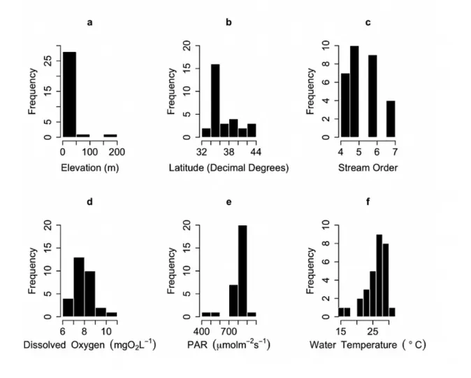
The river observatory stations used in this study sprawled across the entire archipelago from Hokkaido to Kyushu (Fig. 2; Table 1). The elevation of the observatory stations ranged from 1 m at the Shinano River to 181 m at the Kitakami River (Fig. 4; Table 1). The rivers examined were mid to large sized, with stream orders ranging from 4 to 7 (Table 1). Mean DO concentration in August ranged from 4.90 to 10.58 mg O2 /L and that of PAR ranged from 457 to 1062 μmol m-2 s -1 (Fig. 4; Table 1). Mean water temperature in August ranged from 15.3 ℃ at the Toyohira River
to 31.9 ℃ at the Yodo River.
I obtained a total of 646 estimates for each of gross primary production (GPP) and ecosystem respiration (ER), with 110 mean values for August in different years and at different river stations (3-15 data points per river station). Reaeration rates (K) ranged from 0.01 day-1 to 33.87 day-1,
with a mean of 7.33 day-1. GPP rates varied highly, with the estimates ranging from 0.01 g Cm-2
d-1 at the Nagara River (ID = 15, n = 110) to 8.62 g Cm-2 d-1 at the Kiso River (ID = 13, n = 110).
River. Model estimate of K was significantly and positively correlated with both GPP (r = 0.32, p < 0.005) and ER (r = 0.26, p < 0.005) (Fig. 5). Across all river stations, GPP rates covaried positively and significantly with ER rates, although a few rivers, such as the Iwaki River (ID = 5) and the Yamato River (ID = 27), had higher ER rates without correspondingly high GPP rates (Fig. 6; Fig 7). On average, NEP ranged from -2.78 g Cm-2 d-1 at the Yamato River to 1.39 g Cm-2 d-1
at the Mimi River (ID = 30), and only 11 out of 30 rivers had positive NEP (Table 3; Fig. 6). GLMM showed that latitude affected significantly GPP and ER but not NEP (Table 3). In simple regression analyses, GPP rate was marginally and ER rate was significantly higher in rivers at higher latitude (Fig. 8a, 8b), while no significant relationship was detected between NEP rate and latitude (Fig. 8c).
To test the generalities of the latitudinal trends found in Japanese rivers, I complied and examined GPP and ER rates in rivers located from 18°N to ~78°N that were estimated in 27 previous studies (Table 2). Both GPP and ER rates from literature and in this study ranged from 0 to 20 g C m-2 d-1. In addition, the literature data showed that GPP and ER increased significantly
towards higher latitude in accord with the trends found in Japanese rivers (Fig 8d, 8e). Similar to Japanese rivers, most of the NEP from literature showed negative rates. In the case of data from literature, NEP tended to show significantly lower rates at the higher latitude (Fig 8f).
Structural equation modelling (SEM) explained 11% and 53% of variations in GPP and ER in Japanese rivers with significant direct and indirect effects of explanatory variables on these metabolic rates (Fig. 9). In the model, latitude had a significant positive direct effect on both GPP (standardized effect = 0.38) and ER (standardized effect = 0.21). Moreover, latitude had a significant indirect effect through negative effects of water temperature on GPP (standardized effect = -0.600.39 = -0.23). Although ER was not directly affected by water temperature, it was
positively related to GPP (standardized effect = 0.69) and negatively related to elevation (standardized effect = -0.18).
PAR also showed a significant positive indirect effect on both GPP (standardized effect = 0.240.39 = 0.09) through water temperature. Latitude had a significant and negative direct effect on NEP (standardized effect = -0.23). However, no significant effects of water temperature were found for NEP. Instead, NEP was positively related to elevation (standardized effect = 0.28).
Discussions
Since both photosynthesis and respiration rates in river ecosystems often depend on water temperature (Bott et al. 1985; Acuña et al. 2004; Uehlinger 2006; Demars et al. 2011; Hunt et al. 2012; Beaulieu et al. 2013; Escoffier et al. 2016), I first hypothesized that both gross primary production (GPP) and ecosystem respiration (ER) would systematically change with latitude. However, as opposed to my hypothesis, both GPP and ER increased along the latitude. To current knowledge, only one previous study (Lamberti and Steinman 1997) examined the relationship between GPP and latitude for rivers between 30°N and 50°N, which failed to find any significant latitudinal effects. Dataset from 27 previous studies that examined rivers between 18°N and 78°N also showed increase in the GPP and ER rates at higher latitude. Therefore, increasing trends of river GPP and ER rates towards the north seems to be limited not only in Japan but occurs on much larger scales. In this study, water temperatures had positive effects on GPP rate in Japanese rivers, which in turn positively affected on ER rate.
Thus, although latitude can indirectly affect both GPP and ER rates through its negative effect on water temperature, other factors related with latitudinal gradients override this indirect effect. Other than temperature and irradiance, vegetation type, biomass, and anthropogenic land uses are known to change along latitude (Dixon et al. 1994; Dong et al. 2003; Clavero et al. 2011).
Thus, positive trends of GPP and ER rates along latitude may be caused by land use and land covers in the river watershed.
Estimation of reaeration rate in rivers is important to properly estimate the ecosystem metabolism (Mulholland et al. 2001). In this study, the reaeration rate was estimated by the BASE v2.0 model using the time series of DO data (Grace et al. 2015; Dodds et al. 2018; Saltarelli et al. 2018). BASE v2.0 is certainly advantageous for estimating reaeration rate and thus river metabolic rates with the statistical reliability. In general, reaeration rates estimated by model equations tend to underestimate compared with those estimated directly by gas tracer methods and empirical equations (Young and Huryn 1999; Mulholland et al. 2001). However, the degree of underestimation by the model equations was found to be small when the reaeration rate was less than 50 day-1 (Young and Huryn 1999) and when the river was deeper than 6 cm (Mulholland et
al. 2001). In this study, river depth was greater than 6 cm, and the estimated reaeration rate ranged from 0.01 day-1 to 33.87 day-1, with a mean of 7.33 day-1, within the range of values reported in
previous studies (Young and Huryn 1999; Griffiths et al. 2013). Because I used a DO dataset measured at hourly intervals, my estimates of reaeration rates and metabolic rates might be sensitive to the precision of the data points. To increase the accuracy of the estimation of GPP and ER, I used the mean of the daily estimates of metabolic rates for at least three days during August as a single data point. The estimates of gross primary production rate (0.01 to 8.62 g Cm-2 d-1) and
ecosystem respiration rate (0.01 to 9.68 g Cm-2 d-1) in this study are within the range of previous
studies, suggesting that the river metabolic rates estimated in this study are reasonable and have not deviated greatly from the true values.
A significant indirect effect of PAR on GPP and ER through water temperature was seen in the SEM (Fig. 9). This presence of an indirect effect of PAR along with the absence of a direct effect of PAR on metabolic values suggest that the effect of light on the bottom of the river could
have been camouflaged by other local factors such as turbidity and cloud cover. In general, the penetration of light to the bottom of a river decreases moving downstream, if all else is equal, because of the increasing water depth. In addition, with increasing stream order, rivers tend to receive more suspended particles and organic matter that increase the attenuation coefficient of light. In this study, I used PAR at the river surface and did not consider the attenuation coefficient of light in the river water (Krause-Jensen and Sand-Jensen 1998; Brandão et al. 2017). Thus, the actual light level received by the autotrophs in rivers may have been not proportional to PAR at the surface.
Summer precipitation is generally lower in the northern areas compared to the southern areas of Japan (Japan Meteorological Agency 2016). Since inflows of nutrients and organic matter into rivers are expected to be higher in areas with greater precipitation, GPP and ER would be expected to be greater towards the south. However, as shown above, such latitudinal gradients in the metabolic rates were not found. The vegetation types also differ between northern and southern Japan (Numata et al. 1972). For example, broad-leaved evergreen trees dominate the southern region, whereas coniferous trees and broad-leaved deciduous trees are predominant in the northern region. In addition, central and southern Japan are more urbanized and sustain greater population density than in the north (UNDESA 2012). Such latitudinal differences in land use and land cover may have directly or indirectly confounded the latitudinal trends in GPP and ER. Finer spatial analysis on the watershed would be essential to uncover the actual mechanisms of the effects of land cover and land use on river metabolism.
Among the 30 rivers examined in Japan, only 11 rivers showed positive NEP, indicating that most of these rivers are net heterotrophic in the summer, as has been reported in various rivers in other continents (Roberts et al. 2007; Beaulieu et al. 2013; Escoffier et al. 2016; Hall et al. 2016; Kupilas et al. 2017; Rovelli et al. 2017). In this study, I hypothesized that river ecosystems are
more heterotrophic in rivers located at lower latitude since ER is more sensitive to changes in temperature than GPP (Allen et al. 2005; Song et al. 2018). However, opposite to the hypothesis, both in regional (Japanese rivers) and global scales, NEP showed lower values in rivers at higher latitudes. Since this spatial trend cannot be explained by temperature, it may reflect higher allochthonous input relative to primary production in northern rivers. This study also showed that elevation had a significant positive direct effect on NEP, with rivers at lower elevations exhibiting lower NEP than rivers further above sea level. These results suggest that the ecosystem respiration rate relative to primary production rate increased moving downstream, where more allochthonous organic matter from the upstream areas or the surrounding watersheds tends to accumulate. Previous studies (Cole and Caraco 2001; Iwata et al. 2013) also showed that downstream export of greater amounts of organic matter fuels heterotrophic respiration in rivers.
This study explained at most 11% and 53% of the spatial variation in summer GPP and ER rates of rivers in Japan through the direct and indirect effects of latitude, PAR and water temperature and elevation, indicating factors other than geographic position play pivotal roles in determining river metabolism. The development of epilithic algal biomass on riverbeds is a crucial determinant of GPP and depends highly on temporal variability in the flow rate of river waters (Allan and Castillo 2007). The supply of nutrients associated with watershed anthropogenic activities also influences the algal biomass in rivers (Castillo 2010; Miura and Urabe 2017). ER in rivers is also affected by the allochthonous supply of organic matter from agricultural and urban areas and riparian forests (Marcarelli et al. 2011). Thus, local environmental factors specific to individual rivers, which are related or unrelated to latitudinal gradients, may have masked the effects of the thermal gradient on GPP and ER rates.
In conclusion, although GPP and ER rates increased with increasing river water temperature, my analysis showed increase in GPP and ER rates and decrease in NEP rate toward higher latitudes,
indicating that effects of latitude are not limited to temperature and are likely to include indirect effects of local environmental conditions. I first expected that a comparison of river metabolism along latitudinal gradients may be useful to predict the effects of putative warming on river ecosystems. However, latitudinal trends of GPP, ER and NEP found in this study suggest that the uniqueness of each river in conjunction with the latitudinally related factors such as land use and land cover confound the effects of temperatures on these metabolic rates. Thus, to better understand the effects of warming on river ecosystems, it is important to consider both local and latitudinal environmental conditions including vegetation types and biomass, and anthropogenic activities in the watershed.
References
1. Acuña, V. ., A. . Giorgi, I. . Muñoz, F. . Sabater, and S. . Sabater. 2007. Meteorological and riparian influences on organic matter dynamics in a forested Mediterranean stream. kJ. North Am. Benthol. Soc. 26: 54–69.
doi:10.1899/0887-3593(2007)26[54:MARIOO]2.0.CO;2
2. Acuña, V., A. Giorgi, I. Muñoz, U. Uehlinger, and S. Sabater. 2004. Flow extremes and benthic organic matter shape the metabolism of a headwater Mediterranean stream. Freshw. Biol. 49: 960–971. doi:10.1111/j.1365-2427.2004.01239.x
3. Allan, J. D., and M. M. Castillo. 2007. Stream Ecology: Structure and Function of Running waters, Second Edi.
4. Allen, A. P., J. F. Gillooly, and J. H. Brown. 2005. Linking the global carbon cycle to individual metabolism. Funct. Ecol. 19: 202–213. doi:10.1111/j.1365-2435.2005.00952.x 5. Aristegi, L., O. Izagirre, and A. Elosegi. 2010. Metabolism of Basque streams measured
with incubation chambers. Limnetica 29: 301–310.
6. Atkinson, B. L., M. R. Grace, B. T. Hart, and K. E. N. Vanderkruk. 2008. Sediment instability affects the rate and location of primary production and respiration in a sand-bed stream. J. North Am. Benthol. Soc. 27: 581–592. doi:10.1899/07-143.1
7. Bates, D., M. Maechler, B. Bolker, and S. Walker. 2015. Fitting Linear Mixed-Effects Models Using {lme4}. J. Stat. Softw. 67: 1–48. doi:10.18637/jss.v067.i01
8. Beaulieu, J. J., C. P. Arango, D. A. Balz, and W. D. Shuster. 2013. Continuous monitoring reveals multiple controls on ecosystem metabolism in a suburban stream. Freshw. Biol. 58: 918–937. doi:10.1111/fwb.12097
9. Benson, E. R. 2010. Relationships between ecosystem metabolism, benthic macroinvertebrate desities, and envirnmental variables in a sub-arctic Alaskan River. University of Alaska Fairbanks.
10. Bernot, M. J., D. J. Sobota, R. O. Hall, and others. 2010. Inter-regional comparison of land-use effects on stream metabolism. Freshw. Biol. 55: 1874–1890. doi:10.1111/j.1365-2427.2010.02422.x
11. Betts, E. F., and J. B. Jones. 2009. Impact of Wildfire on Stream Nutrient Chemistry and Ecosystem Metabolism in Boreal Forest Catchments of Interior Alaska. Arctic, Antarct. Alp. Res. 41: 407–417. doi:10.1657/1938-4246-41.4.407
12. Bott, T. L., J. D. Newbold, and D. B. Arscott. 2006. Ecosystem metabolism in piedmont streams: Reach geomorphology modulates the influence of riparian vegetation. Ecosystems 9: 398–421. doi:10.1007/s10021-005-0086-6
13. Bott, T. L., J. T. Brock, C. S. Dunn, R. J. Naiman, R. W. Ovink, and R. C. Petersen. 1985. Benthic Comminity Metabolism Along The River Continuum. Hydrobiologia.
14. Brandão, L. P. M., L. S. Brighenti, P. A. Staehr, F. A. R. Barbosa, and J. F. Bezerra-Neto. 2017. Partitioning of the diffuse attenuation coefficient for photosynthetically available irradiance in a deep dendritic tropical lake. An. Acad. Bras. Cienc. 89: 469–489. doi:10.1590/0001-3765201720160016
15. Cappelletti, C. 2006. Photosynthesis and Respiration in an arctic Tundra River : Modification and Application of the Wholestream metabolism method and the influence of physical, biological, and chemical variables.
16. Castillo, M. M. 2010. Land use and topography as predictors of nutrient levels in a tropical catchment. Limnologica 40: 322–329. doi:10.1016/j.limno.2009.09.003
17. Chen, G. 2013. Ecosystem oxygen metabolism in an impacted temperate river network: Application of the δ18O-DO approach.
18. Clavero, M., D. Villero, and L. Brotons. 2011. Climate change or land use dynamics: Do we know what climate change indicators indicate? PLoS One 6.
doi:10.1371/journal.pone.0018581
19. Cole, J. J., and N. F. Caraco. 2001. Carbon in catchments: Connecting terrestrial carbon losses with aquatic metabolism. Mar. Freshw. Res. 52: 101–110. doi:10.1071/MF00084 20. Coon, W. F. 1997. Estimation of roughness coefficients for natural stream channels with
vegetated banks,.
21. Davies, C. J., C. H. Fritsen, E. D. Wirthlin, and J. C. Memmott. 2012. High rates of primary productivity in a semi-arid tailwater: Implications for self-regulated production. River Res. Appl. 21: 1820–1829. doi:10.1002/rra
22. Demars, B. O. L., J. Russell Manson, J. S. Ólafsson, and others. 2011. Temperature and the metabolic balance of streams. Freshw. Biol. 56: 1106–1121. doi:10.1111/j.1365-2427.2010.02554.x
23. Demars, B. O. L., G. M. Gíslason, J. S. Ólafsson, J. R. Manson, N. Friberg, J. M. Hood, J. J. D. Thompson, and T. E. Freitag. 2016. Impact of warming on CO2emissions from streams countered by aquatic photosynthesis. Nat. Geosci. 9: 758–761. doi:10.1038/ngeo2807
24. Dixon, R. K., S. Brown, R. A. Houghton, A. M. Solomon, M. C. Trexler, and J. Wisniewski. 1994. Carbon pools and flux of global forest ecosystems. Science (80-. ). 263: 185–190. doi:10.1126/science.263.5144.185
25. Dodds, W. K., S. A. Higgs, M. J. Spangler, and others. 2018. Spatial heterogeneity and controls of ecosystem metabolism in a Great Plains river network. Hydrobiologia 813: 85– 102. doi:10.1007/s10750-018-3516-0
26. Dong, J., C. Tucker, W. Buermann, R. Kaufmann, and M. Hughs. 2003. USDA Forest Service / UNL Faculty Remote Sensing Estimates of Boreal and Temperate Forest Woody Biomass : Carbon Pools , Sources , and Sinks carbon pools , sources , and sinks. Remote Sens. Environ. 84: 393–410.
27. Duffer, W. R., and T. C. Dowis. 1966. OCEANOGRAPHY.
28. Escoffier, N., N. Bensoussan, L. Vilmin, N. Flipo, V. Rocher, A. David, F. Métivier, and A. Groleau. 2016. Estimating ecosystem metabolism from continuous multi-sensor measurements in the Seine River. Environ. Sci. Pollut. Res. 1–17. doi:10.1007/s11356-016-7096-0
29. ESRI. 2017. Environmental Systems Research Institute.
30. Fellows, C. S., H. M. Valett, C. N. Dahm, P. J. Mulholland, and S. A. Thomas. 2006. Coupling nutrient uptake and energy flow in headwater streams. Ecosystems 9: 788–804. doi:10.1007/s10021-006-0005-5
31. Finlay, J. C. 2011. Stream size and human influences on ecosystem production in river networks. Ecosphere 2: art87. doi:10.1890/ES11-00071.1
32. Flemer, D. A. 1970. Primary productivity of the North Branch of the Raritan River, New Jersey. Hydrobiologia 35: 273–296. doi:10.1007/BF00181732
33. Grace, M., and S. Imberger. 2006. Stream Metabolism : Performing & Interpreting Measurements. New South Wales Dep. Environ. Conserv. Stream Metab. Work. May 31: 204. doi:10.4296/cwrj3101041
34. Grace, M. R., D. P. Giling, S. Hladyz, V. Caron, R. M. Thompson, and R. Mac Nally. 2015. Fast processing of diel oxygen curves: Estimating stream metabolism with base (BAyesian single-station estimation). Limnol. Oceanogr. Methods 13: 103–114. doi:10.1002/lom.10011
J. Beaulieu, and L. T. Johnson. 2013. Agricultural land use alters the seasonality and magnitude of stream metabolism. Limnol. Oceanogr. 58: 1513–1529. doi:10.4319/lo.2013.58.4.1513
36. Hall R. O., J., J. L. Tank, and M. F. Dybdahl. 2003. Exotic snails dominate nitrogen and carbon cycling in a highly productive stream. Frontiers in Ecology and the Environment 1(8):407--411. 2.
37. Hall, R. O., and J. L. Tank. 2003. Ecosystem metabolism controls nitrogen uptake in streams in Grand Teton National Park, Wyoming. Limnol. Oceanogr. 48: 1120–1128. doi:10.4319/lo.2003.48.3.1120
38. Hall, R. O., J. L. Tank, M. A. Baker, E. J. Rosi-Marshall, and E. R. Hotchkiss. 2016. Metabolism, Gas Exchange, and Carbon Spiraling in Rivers. Ecosystems 19: 73–86. doi:10.1007/s10021-015-9918-1
39. Hart, A. M. 2013. Seasonal Variation in Whole Stream Metabolism across Varying Land Use Types Adam Michael Hart Thesis submitted to the faculty of the Virginia Polytechnic Institute and State University in partial fulfillment of the requirements for the degree of Master of. 66.
40. Holtgrieve, G. W., D. E. Schindler, T. A. Branch, and Z. T. A’mar. 2010. Simultaneous quantification of aquatic ecosystem metabolism and reaeration using a Bayesian statistical model of oxygen dynamics. Limnol. Oceanogr. 55: 1047–1063. doi:10.4319/lo.2010.55.3.1047
41. Hotchkiss, E. R., R. O. Hall Jr, R. A. Sponseller, D. Butman, J. Klaminder, H. Laudon, M. Rosvall, and J. Karlsson. 2015. Sources of and processes controlling CO2 emissions change with the size of streams and rivers. Nat. Geosci. 8: 696–699. doi:10.1038/ngeo2507 42. Hunt, R. J., T. D. Jardine, S. K. Hamilton, and S. E. Bunn. 2012. Temporal and spatial variation in ecosystem metabolism and food web carbon transfer in a wet-dry tropical river. Freshw. Biol. 57: 435–450. doi:10.1111/j.1365-2427.2011.02708.x
43. Iwata, T., T. Takahashi, F. Kazama, and others. 2007. Metabolic balance of streams draining urban and agricultural watersheds in central Japan. Limnology 8: 243–250. doi:10.1007/s10201-007-0212-6
44. Iwata, T., T. Suzuki, H. Togashi, N. Koiwa, H. Shibata, and J. Urabe. 2013. Fluvial transport of carbon along the river-to-ocean continuum and its potential impacts on a brackish water food web in the Iwaki River watershed, northern Japan. Ecol. Res. 28: 703– 716. doi:10.1007/s11284-013-1047-8
45. Iyama, S. 1993. Profile of Japanese Rivers - Background to River Engineering in Japan. J. Hydrosci. Hydraul. Eng. 1–4.
46. Japan Meteorological Agency. 2016. Climate Change Monitoring Report 2015.
47. Kaenel, B. R., H. Buehrer, and U. Uehlinger. 2000. Effects of aquatic plant management on stream metabolism and oxygen balance streams. Freshw. Biol. 45: 85–95. doi:10.1046/j.1365-2427.2000.00618.x
48. Kosinski, R. J. 1984. A comparision of the accuracy and precision of several open-water oxygen productivity techniques.
49. Krause-Jensen, D., and K. Sand-Jensen. 1998. Light attenuation and photosynthesis of aquatic plant communities. Limnol. Oceanogr. 43: 396–407.
doi:10.4319/lo.1998.43.3.0396
50. Kupilas, B., D. Hering, A. Lorenz, C. Knuth, and B. Gucker. 2017. Hydromorphological restoration stimulates river ecosystem metabolism. Biogeosciences 14: 1989–2002. doi:10.5194/bg-14-1989-2017
ecosystems. J. North Am. Benthol. Soc. 16: 95–103.
52. Marcarelli, A. M., C. V. Baxter, M. M. Mineau, and R. O. Hall. 2011. Quantity and quality: Unifying food web and ecosystem perspectives on the role of resource subsidies in freshwaters. Ecology 92: 1215–1225. doi:10.1890/10-2240.1
53. Masese, F. O., J. S. Salcedo-Borda, G. M. Gettel, K. Irvine, and M. E. McClain. 2017. Influence of catchment land use and seasonality on dissolved organic matter composition and ecosystem metabolism in headwater streams of a Kenyan river. Biogeochemistry 132: 1–22. doi:10.1007/s10533-016-0269-6
54. Miura, A., and J. Urabe. 2017. Changes in epilithic fungal communities under different light conditions in a river: A field experimental study. Limnol. Oceanogr.
55. Mulholland, P. J., C. S. Fellows, J. L. Tank, and others. 2001. Inter-biome comparison of factors controlling stream metabolism. Freshw. Biol. 46: 1503–1517. doi:10.1046/j.1365-2427.2001.00773.x
56. Naegeli, M. W., and U. Uehlinger. 1997. Contribution of the hyporheic zone to ecosystem metabolism in a prealpine gravel-bed river. J. North Am. Benthol. Soc. 16: 794–804. 57. Naiman, R. J. 1983. The annual pattern and spatial distribution of aquatic oxygen
metabolism in boreal forest watershed. Ecol. Monogr. 53(1): 73–94. doi:https://doi.org/10.2307/1942588
58. Numata, M., A. Miyawaki, and D. Itow. 1972. Natural and semi-natural vegetation in Japan. Blumea 20: 435–481.
59. R Core Team. 2014. R: A Language and Environment for Statistical Computing.
60. Rasmussen, J. J., A. Baattrup-Pedersen, T. Riis, and N. Friberg. 2011. Stream ecosystem properties and processes along a temperature gradient. Aquat. Ecol. 45: 231–242. doi:10.1007/s10452-010-9349-1
61. Roberts, B. J., P. J. Mulholland, and W. R. Hill. 2007. Multiple scales of temporal variability in ecosystem metabolism rates: Results from 2 years of continuous monitoring in a forested headwater stream. Ecosystems 10: 588–606. doi:10.1007/s10021-007-9059-2
62. Rosseel, Y. 2012. {{lavaan}: An {R} Package for Structural Equation Modeling}. J. Stat. Softw. 48: 1–36. doi:10.18637/jss.v048.i02
63. Rovelli, L., K. M. Attard, A. Binley, C. M. Heppell, H. Stahl, M. Trimmer, and R. N. Glud. 2017. Reach-scale river metabolism across contrasting sub-catchment geologies: Effect of light and hydrology. Limnol. Oceanogr. 62: S381–S399. doi:10.1002/lno.10619
64. Saltarelli, W. A., W. K. Dodds, F. Tromboni, M. do C. Calijuri, V. Neres-Lima, C. E. Jordao, P. J. C.P, and D. G. F. Cunha. 2018. Variation of stream metabolism along a tropical environmental gradient. J. Limnol. doi:10.4081/jlimnol.2018.
65. Song, C., W. K. Dodds, J. Rüegg, and others. 2018. Continental-scale decrease in net primary productivity in streams due to climate warming. Nat. Geosci. 11. doi:10.1038/s41561-018-0125-5
66. Uehlinger, U. 2006. Annual cycle and inter-annual variability of gross primary production and ecosystem respiration in a floodprone river during a 15-year period. Freshw. Biol. 51: 938–950. doi:10.1111/j.1365-2427.2006.01551.x
67. UNDESA. 2012. World Urbanization Prospects: The 2011 Revision. Present. Cent. Strateg. … 318. doi:10.2307/2808041
68. Webster, J. R., J. B. Wallace, and E. F. Benfield. 1995. Organic processes in streams of the eastern United States. River stream Ecosyst. world 117–187. doi:citeulike-article-id:6945780
70. Yanai, S. 2008. Sediment dynamics and characteristics with respect to river disturbance, p. 31–45. In T. Sakio, Hitoshi; Tamura [ed.], Ecology of Riparian Forests in Japan.
71. Yoshimura, C., T. Omura, H. Furumai, and K. Tockner. 2005. Present state of rivers and streams in Japan. River Res. Appl. 21: 93–112. doi:10.1002/rra.835
72. Young, R. G., and A. D. Huryn. 1999. Effects of Land Use on Stream Metabolism and Organic Matter Turnover. Ecol. Appl. 9: 1359–1376.
73. Young, R. G., C. D. Matthaei, and C. R. Townsend. 2008. Organic matter breakdown and ecosystem metabolism: functional indicators for assessing river ecosystem health. J. North Am. Benthol. Soc. 27: 605–625. doi:10.1899/07-121.1
Fig. 1. Examples of patterns of diel dissolved oxygen (DO) data. (a) and (b) show examples of the distinct diel patterns that were included in the study, whereas erratic and inconsistent sites such as (c) were excluded. (a) Chikuko River, August 2012; (b) Shonai River, August 2016; and (c) Kitakami River, August 2015.
Fig. 2. Map of Japan showing the river observatory stations where the dissolved oxygen (DO) and water temperature data were collected. Details of each river are shown in Table 2.
Fig. 3. Example of validation plots for Ginbashi on the Ina River in Aug 4, 2015, obtained after running the model. Upon a successful convergence of the model, all five chains (A, p, R, K.day and theta) overlap and become centred. Plots of measured dissolved oxygen (DO) (empty circle) and predicted DO (black line), and measured temperature and photosynthetically active radiation (PAR) data are shown for each diel period.
Fig. 4. Frequency histogram of independent parameters used in the study. (a) Elevation, (b) Latitude, (c): Stream Order, (d): Dissolved Oxygen (DO), (e): Photosynthetically Active Radiation (PAR) and (f) Water temperature.
Fig. 5. Relationship between gross primary production (GPP) rate and ecosystem respiration (ER) and reaeration rate in the Japanese rivers.
Fig. 6. River metabolic rates along the latitudinal gradient in Japan. The x-axis shows latitude (from the south to the north), and the y-axis shows gross primary production (GPP) rate (upper panel), ecosystem respiration (ER) rate (mid panel) and net ecosystem production (NEP) (lower panel) in units of carbon.
Fig. 7. Relationship between gross primary production rate (GPP) and ecosystem respiration rate (ER) across the rivers examined in Japan. Data points are rates estimated in single years.
Horizontal and vertical bars are standard errors of GPP and ER, respectively. Thick line and grey area represent the regression line with 95% confidence intervals. Dashed line indicates 1:1 line.
Fig. 8. Gross primary production rate (GPP), ecosystem respiration rate (ER) and net ecosystem production (NEP) rate of the rivers in Japan (a, b & c: regional scale) and various areas (d, e & f: global scale) plotted against latitude. The results of GLMM with the statistical values are shown in Table 4.
Fig. 9. Results of the structural equation model, showing direct and the indirect effects of latitude and other factors on gross primary production (GPP) rate, ecosystem respiration (ER) rate and net ecosystem production (NEP) rate of the rivers in Japan. Strengths of effects are denoted by path coefficients (i.e., regression coefficients). Red and blue lines indicate significantly negative and positive paths (p < 0.05), respectively, and dashed lines indicate hypothesized pathways that were not significant in the model. The amount of variation explained by the model is given by R2 with
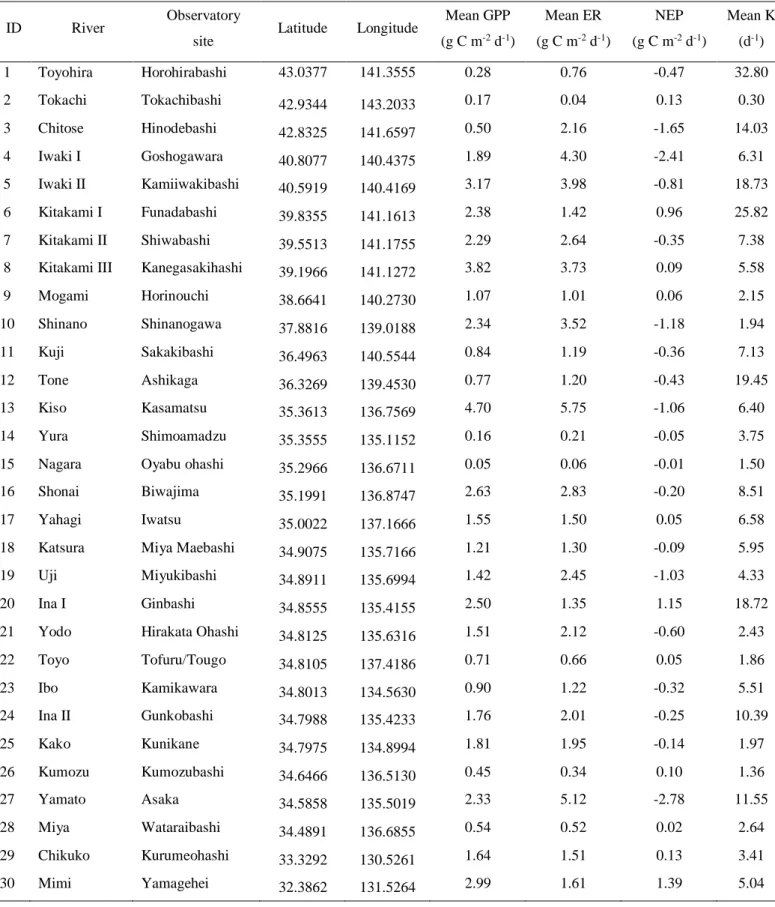
Table 1. Geographical positions and details of the observatory sites of the Japanese rivers used in this study.
ID River Observatory Site Latitude Longitude Stream Order Elevation (m) Depth (m) Mean water temperature (°C)
Max diel PAR (μ mol m-2 s-1) Mean DO (mg O2/l) 1 Toyohira Horohirabashi 43.0377 141.3555 5 32 0.62 15.33 472.30 9.93 2 Tokachi Tokachibashi 42.9344 143.2033 6 19 1.02 17.68 748.31 10.58 3 Chitose Hinodebashi 42.8325 141.6597 4 10 0.15 20.64 577.75 8.61 4 Iwaki I Goshogawara 40.8077 140.4375 6 10 1.04 22.01 826.86 7.57 5 Iwaki II Kamiiwakibashi 40.5919 140.4169 4 45 0.57 23.32 751.69 8.25 6 Kitakami I Funada bashi 39.8355 141.1613 5 181 0.51 20.94 802.66 8.91 7 Kitakami II Shiwabashi 39.5513 141.1755 6 92 0.96 24.39 730.34 7.98 8 Kitakami III Kanegasaki hashi 39.1966 141.1272 7 41 1.35 25.12 756.36 8.04 9 Mogami Horinouchi 38.6641 140.2730 6 49 1.44 26.42 801.17 8.33 10 Shinano Shinanogawa 37.8816 139.0188 7 1 2.33 27.20 877.46 7.76 11 Kuji Sakakibashi 36.4963 140.5544 5 9 0.39 27.68 895.13 7.57 12 Tone Ashikaga 36.3269 139.4530 5 40 0.26 25.50 842.70 7.82 13 Kiso Kasamatsu 35.3613 136.7569 6 10 0.95 25.25 847.92 7.18 14 Yura Shimoamadzu 35.3555 135.1152 6 16 0.40 28.72 868.41 7.52 15 Nagara Ōyabu ōhashi 35.2966 136.6711 6 10 0.16 25.85 893.90 8.27 16 Shōnai Biwajima 35.1991 136.8747 5 11 0.48 29.52 807.07 7.28 17 Yahagi Iwatsu 35.0022 137.1666 5 27 0.61 27.01 815.88 7.86 18 Katsura Miya Maebashi 34.9075 135.7166 6 14 0.41 28.68 787.89 7.34 19 Uji Miyukibashi 34.8911 135.6994 6 11 1.28 29.70 812.61 6.91 20 Ina I Ginbashi 34.8555 135.4155 4 11 0.27 28.82 808.08 8.11 21 Yodo Hirakata Ōhashi 34.8125 135.6316 7 2 1.25 30.73 834.93 6.90 22 Toyo Tō furu/Tougo 34.8105 137.4186 4 9 0.30 27.35 789.05 8.03 23 Ibo Kamikawara 34.8013 134.5630 5 4 0.44 27.91 968.78 7.37 24 Ina II Gunkōbashi 34.7988 135.4233 4 12 0.24 27.65 832.25 7.19 25 Kako Kunikane 34.7975 134.8994 6 13 0.38 28.88 829.35 6.83 26 Kumozu Kumozubashi 34.6466 136.5130 4 6 0.26 28.03 802.07 8.69 27 Yamato Asaka 34.5858 135.5019 5 6 0.45 29.67 844.73 6.10 28 Miya Watarai-bashi 34.4891 136.6855 5 10 0.43 26.92 727.88 7.93 29 Chikuko Kurumeōhashi 33.3292 130.5261 7 2 0.65 27.67 871.12 8.92 30 Mimi Yamagehei 32.3862 131.5264 4 19.3 1.2 22.52 857.73 9.20
Table 2. GPP and ER rates in summer of various rivers estimated in previous studies.
Citation Name of river Latitude GPP (g C m-2 d-1) ER (g C m-2 d-1)
Aristegi et al. (2009) Aitzu 43.026111 10.43 4.43
Aristegi et al. (2009) Aizarnazabal 43.026111 0.71 1.01
Aristegi et al. (2009) Alegia 43.026111 6.86 6.45
Aristegi et al. (2009) Altzola 43.026111 13.24 2.36
Aristegi et al. (2009) Amorebieta 43.026111 4.09 1.39
Aristegi et al. (2009) Balmaseda 43.026111 3.19 3.83
Aristegi et al. (2009) Berriatua 43.026111 2.10 1.13
Aristegi et al. (2009) Elorrio 43.026111 1.50 1.46
Aristegi et al. (2009) Erenozu 43.026111 4.20 3.75
Aristegi et al. (2009) Estanda 43.026111 1.24 0.49
Aristegi et al. (2009) Gardea 43.026111 3.49 4.73
Aristegi et al. (2009) Herrerias 43.026111 3.56 1.39
Aristegi et al. (2009) Lasarte 43.026111 3.64 3.71
Aristegi et al. (2009) Leitzaran 43.026111 2.06 3.30
Aristegi et al. (2009) Muxika 43.026111 3.23 2.06
Aristegi et al. (2009) Oiartzun 43.026111 0.68 0.41
Aristegi et al. (2009) Olet 43.026111 5.33 4.01
Aristegi et al. (2009) Onati 43.026111 5.78 2.10
Aristegi et al. (2009) S.Prudentzio 43.026111 4.09 2.51
Aristegi et al. (2009) Sodupe 43.026111 0.00 3.00
Benson (2010) Site 4 64.804217 0.74 1.58 Benson (2010) Site 4 64.804217 0.70 2.46 Benson (2010) Site 3 64.817533 0.62 1.91 Benson (2010) Site 3 64.817533 0.77 2.68 Benson (2010) Site 2 64.880783 0.81 1.89 Benson (2010) Site 2 64.880783 0.72 2.43 Benson (2010) Site 1 64.898483 1.47 3.35 Benson (2010) Site 1 64.898483 0.97 3.36
Bernot et al. (2010) Grande 18.16 1.95 2.85
Bernot et al. (2010) Maizales 18.23 2.74 1.99
Bernot et al. (2010) Ceiba 18.27 3.49 4.39
Bernot et al. (2010) RIT 18.28 0.19 1.69
Bernot et al. (2010) Bisley 18.32 0.02 0.90
Bernot et al. (2010) Pared 18.33 0.15 0.15
Bernot et al. (2010) Vaca 18.34 1.16 5.89
Bernot et al. (2010) Mtrib 18.37 2.66 2.78
Bernot et al. (2010) Petunia 18.39 0.11 1.73
Bernot et al. (2010) Sycamore Ck 33.75 1.05 1.46
Bernot et al. (2010) Blacks Branch 34.94 0.19 3.26
Bernot et al. (2010) Jerry Branch 34.96 0.19 1.69
Bernot et al. (2010) Hugh White Creek 35.05 0.04 0.83
Bernot et al. (2010) Cunningham Creek 35.05 0.02 1.95
Bernot et al. (2010) Hoglot Branch 35.09 0.11 0.60
Bernot et al. (2010) Crawford Branch 35.18 1.13 2.44
Bernot et al. (2010) Rio Rancho 35.2 2.44 3.75
Bernot et al. (2010) San Pedro 35.21 1.24 1.99
Bernot et al. (2010) Bernalillo drain 35.33 3.30 2.66
Bernot et al. (2010) Sugarloaf Creek 35.38 0.04 6.71
Bernot et al. (2010) Kings Creek N4D 39.09 0.68 1.16
Bernot et al. (2010) Campus Creek 39.19 0.11 0.19
Bernot et al. (2010) Agnorth 39.21 3.00 2.85
Bernot et al. (2010) Natalie Creek 39.23 0.08 0.41
Bernot et al. (2010) Arcadia 42.27 0.30 5.29
Bernot et al. (2010) Honeysuckle 42.31 0.04 2.96
Bernot et al. (2010) Sawmill Brook 42.52 0.02 0.45
Bernot et al. (2010) IS_104 42.54 0.26 3.41
Bernot et al. (2010) Sand Creek 42.58 0.08 0.75
Bernot et al. (2010) IS_118 42.58 0.04 1.50
Bernot et al. (2010) Boxford 42.64 0.02 5.48
Bernot et al. (2010) Black Brook 42.64 0.23 1.69
Bernot et al. (2010) Runaway Brook 42.65 2.74 4.13
Bernot et al. (2010) Long Meadow Brook 42.65 1.46 3.08
Bernot et al. (2010) Gravelly Brook 42.66 0.08 4.24
Bernot et al. (2010) Wayland 42.67 0.68 1.54
Bernot et al. (2010) Steinke Drain 42.71 0.30 0.49
Bernot et al. (2010) Dorr 42.73 0.26 3.26
Bernot et al. (2010) Cart Creek 42.77 0.08 1.43
Bernot et al. (2010) Teton Pines 43.53 1.01 0.56
Bernot et al. (2010) Giltner 43.55 6.08 4.28
Bernot et al. (2010) Golf 43.57 1.58 3.75
Bernot et al. (2010) Kimball 43.57 5.10 4.50
Bernot et al. (2010) Headquarters 43.57 1.24 2.66
Bernot et al. (2010) Ditch 43.66 1.05 1.50
Bernot et al. (2010) Spread 43.79 1.20 3.68
Bernot et al. (2010) Two Oceans 43.88 1.09 4.73
Bernot et al. (2010) Amazon 44.04 1.05 1.84
Bernot et al. (2010) Camp 44.12 0.11 1.84
Bernot et al. (2010) Mack 44.22 0.08 1.80
Bernot et al. (2010) Potts 44.26 0.11 5.36
Bernot et al. (2010) Courtney 44.36 1.13 1.50
Bernot et al. (2010) Oak 44.56 0.30 2.59
Bernot et al. (2010) Oak 44.57 0.38 0.38
Bernot et al. (2010) Oak 44.61 0.15 0.38
Betts and Jones (2009) C2 65.16 0.56 1.69
Betts and Jones (2009) C4 65.16 0.11 0.45
Betts and Jones (2009) P6 burned 65.16 1.13 2.48
Bott et al. (2006) Buck and Doe run, Meadow 39.921389 2.44 3.12
Bott et al. (2006) Buck and Doe Run, Forest 39.925556 0.55 1.14
Bott et al. (2006) Big Springs, Forest 39.930278 0.20 1.96
Bott et al. (2006) Birch Run, Forest 39.930278 0.23 2.04
Bott et al. (2006) Doe Wister, Forest 39.9025 0.62 1.85
Bott et al. (2006) Fishers, Forest 39.928889 0.38 1.24
Bott et al. (2006) Gramies, Forest 39.688333 0.44 0.99
Bott et al. (2006) Hannums, Forest 39.899167 0.19 1.17
Bott et al. (2006) Moorheads, Forest 39.880833 0.03 2.01
Bott et al. (2006) Pocopson, Forest 39.903333 0.67 1.01
Bott et al. (2006) Teters, Forest 39.874722 0.10 0.90
Bott et al. (2006) West Branch WC Cr, Meadow 39.767778 0.44 1.19
Bott et al. (2006) Wests, Forest 39.898333 0.01 1.24
Bott et al. (2006) White Clay Cr, Forest 39.863056 0.69 1.17
Bott et al. (2006) Big Springs, Meadow 39.931944 0.81 2.79
Bott et al. (2006) Birch run, Meadow 39.931944 1.34 1.61
Bott et al. (2006) Doe Wister, Meadow 39.903889 1.99 1.90
Bott et al. (2006) Fishers, Meadow 39.927778 0.81 1.15
Bott et al. (2006) Grammies, Meadow 39.684722 1.95 2.24
Bott et al. (2006) Hannums, Meadow 39.900833 0.62 2.93
Bott et al. (2006) Moorheads, Meadow 39.876944 1.28 2.49
Bott et al. (2006) Pocopson, Meadow 39.903056 0.98 1.46
Bott et al. (2006) Teters, Meadow 39.872222 0.77 2.84
Bott et al. (2006) West Branch WC Cr, Forest 39.7675 0.09 0.67
Bott et al. (2006) Wests, Meadow 39.900556 0.30 2.43
Bott et al. (2006) White clay cr, Meadow 39.768889 0.75 1.04
Bott et al. (2006) Kisco 41.196389 0.08 0.30
Bott et al. (2006) Croton 41.210171 0.45 2.25
Bott et al. (2006) Cross 41.26 0.34 1.13
Bott et al. (2006) Muscoot 41.2694 0.15 0.94
Bott et al. (2006) Neversink 41.357222 0.94 3.00
Bott et al. (2006) Rondout 41.92 1.31 1.50
Bott et al. (2006) Esopus 42.015556 1.46 3.00
Bott et al. (2006) Bushkill 42.14746 1.58 3.00
Bott et al. (2006) West Branch Deleware 42.453611 1.20 1.88
Bott et al. (2006) Schoarie 42.941111 0.79 1.50
Cappelletti (2006) Kuparuk River, Ref 68.633333 0.56 6.75
Cappelletti (2006) Kuparuk River, Fertilized 68.633333 1.05 7.13
Chen (2013) WM 43.052222 4.37 4.62
Chen (2013) GM 43.277228 4.76 4.23
Chen (2013) BL 43.386056 6.76 11.29 Chen (2013) BL 43.386056 6.43 8.71 Chen (2013) BL 43.386056 3.59 7.12 Chen (2013) BP 43.481861 2.61 2.58 Chen (2013) BP 43.481861 2.98 2.13 Chen (2013) BP 43.481861 3.01 2.32 Chen (2013) SPb 43.484236 4.04 4.06 Chen (2013) SPb 43.484236 3.41 3.41 Chen (2013) Spa 43.534567 0.26 0.34 Chen (2013) Spa 43.534567 0.19 0.19 Chen (2013) 5F 43.640064 1.67 2.64 Chen (2013) 5F 43.640064 0.80 1.23 Chen (2013) 5NF 43.666628 3.35 3.41 Chen (2013) 3NF 43.699914 1.25 2.48 Chen (2013) 3NF 43.699914 1.20 2.94 Chen (2013) 4F 43.705731 0.69 1.51 Chen (2013) 4F 43.705731 1.13 2.39 Chen (2013) 4NF 43.707889 0.84 1.27 Chen (2013) 4NF 43.707889 1.16 1.94 Chen (2013) 2NF 43.714703 0.27 1.00 Chen (2013) 2NF 43.714703 0.48 2.10 Chen (2013) 3F 43.7289 1.44 2.23 Chen (2013) 3F 43.7289 0.74 1.27 Chen (2013) 2F 43.734567 0.35 1.40 Chen (2013) 2F 43.734567 0.35 0.93
Davis (2012) South Fork Humboldt 40.666667 5.88 4.02
Demars et al. (2016) PAR 19 52.823583 2.54 7.50
Demars et al. (2016) PAR 21 52.82375 1.02 7.88
Demars et al. (2016) PAR 10 52.824361 1.92 3.83
Demars et al. (2016) PAR 14 52.8245 0.75 2.14
Demars et al. (2016) TOR 2 63.933389 0.09 0.15
Demars et al. (2016) TOR 1 63.933444 1.39 2.40
Demars et al. (2016) TOR 3 63.934389 4.72 4.43
Demars et al. (2016) TOR 4 63.935194 0.78 2.10
Demars et al. (2016) TOR 7 63.954556 3.05 4.58
Demars et al. (2016) TOR 6 63.955028 0.54 0.56
Demars et al. (2016) HG 18 64.009833 5.67 6.30 Demars et al. (2016) HG 19 64.010306 9.39 13.05 Demars et al. (2016) HG 20 64.010833 13.32 17.33 Demars et al. (2016) HG 21 64.011056 16.38 19.20 Demars et al. (2016) HG 37 64.012222 3.23 6.37 Demars et al. (2016) HG 27 64.012806 1.64 1.50 Demars et al. (2016) HG 22 64.018167 5.26 4.05 Demars et al. (2016) HG 23 64.018167 3.69 1.35
Demars et al. (2016) HG 24 64.019056 4.91 3.75 Demars et al. (2016) HG 35 64.025583 6.41 15.93 Demars et al. (2016) HG 36 64.02625 8.22 6.48 Demars et al. (2011) 1 64.05 7.61 10.57 Demars et al. (2016) HG 25 64.059389 0.79 1.38 Demars et al. (2016) HG 26 64.060111 6.68 16.08
Demars et al. (2016) HEN 12 64.080028 1.58 4.28
Demars et al. (2016) HEN 1 64.089944 7.63 10.58
Demars et al. (2016) HEN 5 64.092694 10.35 14.25
Demars et al. (2016) HEN 2 64.093 5.35 7.05
Demars et al. (2016) HEN 3 64.093917 1.86 6.41
Demars et al. (2016) HEN 4 64.094278 0.84 0.94
Demars et al. (2016) HEN 6 64.094472 6.30 6.86
Demars et al. (2016) HEN 7 64.095639 1.66 2.63
Demars et al. (2016) HEN 8 64.09575 5.11 25.05
Demars et al. (2016) HEN 9 64.096361 5.89 9.56
Demars et al. (2016) HEN 10 64.097194 3.91 8.96
Demars et al. (2016) HEN 11 64.098028 3.47 3.64
Demars et al. (2016) HEN 14 64.100528 0.82 1.54
Demars et al. (2011) 14 64.517778 0.83 1.54
Demars et al. (2016) KER 31 64.64575 0.49 1.16
Demars et al. (2016) VON 4 64.679444 0.94 0.94
Demars et al. (2016) VON 5 64.684083 0.20 0.83
Demars et al. (2016) VON 6 64.686056 0.63 1.20
Demars et al. (2016) VON 7 64.687667 3.34 3.34
Demars et al. (2016) KER 43 64.688167 0.73 8.21
Demars et al. (2016) KER 42 64.689472 0.41 2.66
Demars et al. (2016) VON 1 64.6895 3.08 3.64
Demars et al. (2016) VON 8 64.689528 0.38 0.15
Demars et al. (2016) KER 41 64.689556 1.04 3.83
Demars et al. (2016) VON 2 64.690694 1.11 2.10
Demars et al. (2016) KER 40 64.692361 2.52 20.29
Demars et al. (2016) KVE 50 64.865778 1.53 1.84
Demars et al. (2016) KVE 51 64.865861 0.65 1.54
Demars et al. (2011) 5 73.368056 10.35 14.25 Demars et al. (2011) 2 73.66 5.36 7.05 Demars et al. (2011) 3 74.58 1.84 6.41 Demars et al. (2011) 4 74.9347 0.83 0.94 Demars et al. (2011) 6 75.151389 6.30 6.86 Demars et al. (2011) 7 76.301389 1.65 2.63 Demars et al. (2011) 8 76.418056 5.10 25.05 Demars et al. (2011) 9 77.03472 5.89 9.56 Demars et al. (2011) 12 77.351111 1.58 4.28 Demars et al. (2011) 10 78.684722 3.90 8.96