Dynamic Simulation for Domestic Solid Waste Composting Processes

Dynamic Simulation for Domestic Solid Waste Composting Processes

Beidou Xi

, Zimin Wei

, Hongliang Liu

1. Chinese Research Academy of Environmental Sciences, Beijing 100012, China 2. Northeast Agriculture University, Harbin, Heilongjiang 150030, China

[email protected], [email protected]

Abstract: Modeling composting processes is the prerequisite to realize the process control of composting. In this paper, a simulation model for domestic solid waste composting processes was developed based on microbial process kinetics, mass conservation equation, energy conservation equation and water balance. Differential equations describing microbial, substrate, oxygen concentrations, moisture content and temperature profiles were derived.

Considering that several factors (temperature, oxygen, moisture and FAS) in the process interacted to composting processes, microbial biomass growth kinetics was described. In order to verify the model, a series of aerobic composting experiments on domestic solid wastes were conducted. Temperature, moisture, microbial biomass growth, oxygen consumption rate and the concentrations of organic components were monitored in the composting processes and also simulated with the developed model. The simulation results were well consistent with the experimental results. It also could be seen from the model that the efficiency of composting processes could be raised and aeration requirements could be reduced by controlling the oxygen concentration in the exhaust air within a proper range. When the range is 8% to 12%, the aeration requirements reduced 79.61%. This result was verified by the composting experiment. When initial moisture content was higher than 66% or lower than 33%, it would significantly reduce the rate of substrate degradation. It indicated the effect of initial moisture content on the composting processes was significant. A simple sensitivity analysis demonstrated that two key parameters in composting modeling to determine were maximum specific growth rate ( μ

) and yield coefficient (Y

).

Therefore, the composting processes could be optimized by the application of the developed simulation model.

[Academia Arena 2010;2(3):76-89]. (ISSN 1553-992X).

Key words: dynamic simulation; model; composting; domestic solid waste

1. Introduction

The biochemical and physical characteristics of solid wastes (e.g., constituents, pH, and moisture) and operating conditions of solid waste composting (e. g., carbon to nitrogen ratio, aeration rate, reaction temperature and pressure) impose significant effects on an ecological succession of microorganisms (Vallini, 1993; Huang, 2000). Although relationships between these factors have been stressed, it is often difficult to synthesize such a large volume of materials. Generally, the factors that affect composting processes, such as temperature and oxygen availability, are controlled to maintain a relatively better growth environment for microorganisms during the process of composting.

Analytical and numerical modeling of the composting process could be used as a tool to analyze composting system performance under different operating scenarios.

Modeling composting processes is the prerequisite to realize the process control of composting. Over past years, there have been many approaches (Miller, 1996) which have been used to investigate composting processes: (Hammelers, 1993; Stombaugh, 1996;

Agamuthu, 1999) considered growth rates of microorganisms and used the Monod equation to simulate the composting processes (Keener, 1993;

Haug, 1993) made emphasis on the thermodynamic and

kinetic changes taking place during composting

processes. Mohee and White (1998) developed a

dynamic simulation model to present biodegradation

processes in composting based on the knowledge of the

physical and chemical changes occurring in the

processes. Hamoda et al. (1998). Wang and Li (2000)

also conducted a number of works on the modeling for

composting processes. Bari et al. (2000) studied a

kinetics analysis of forced aeration composting processes operated under different aeration modes.

However, at the present, most of the existing composting systems are static control systems and the underlying biological portion of the process has been neglected. At the same time, the states of solid waste are various in different periods due to the dynamic features and the living environment of microorganisms is also incessantly changing due to the increase of metabolizing production and consumption of biochemical reaction.

These inherent complicated processes are insurmountable for design of cost-effective composting system. So, the present models exist some limitation for real composting processes to determine optimal operation conditions. Thus, it is necessary to integrate the intrinsic rate equations with fundamental microbial kinetics to produce a dynamic model of the process. The dynamic simulation model would be more robust than current empirical models. It should consider more complete complexities process of composting and supply interactive relationship of temperature, oxygen, FAS, moisture and microbial biomass growth to instruct the design of composting system and determine the optimal operation conditions for the process.

The primary objective of this study is to develop an integrated simulation model, which can be used for engineering analysis and design. The dynamic kinetics of the whole composting processes and all key factors, which limit the kinetics, will be considered. The model describes substrate degradation, microbial growth, moisture change, oxygen concentration and aeration on- off situation as a function of substrate and oxygen concentration in the exhaust air, compost temperature and moisture content. Realistic economic aeration will be included to evaluate and optimize a rotation vessel composting process with the numerical simulation results. At the same time optimal composting conditions will be identified.

2. Development of dynamic composting of processes simulation model

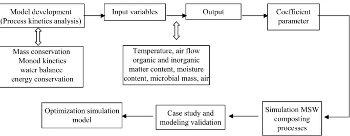
Most modern municipal solid waste composting operations emphasize the enhancement of decomposition rate of the organic matter as well as the economic operating cost. This can be achieved once the composting process kinetics is well understood. Based on microbial process kinetics, mass conservation equation, energy conservation equation and water balance, differential equations describing microbial,

substrate, oxygen concentrations, moisture content and temperature profiles are derived. Then a simulation model for domestic solid waste composting processes is developed. The process is shown in Figure 1.

2.1 Kinetics of composting processes

The complex and dynamic interactions within bioconversion are a fundamental component for developing a proper composting process.

Thermal/physical/chemical interactions must be considered completely in biological and physical composting processes in the simulation modeling. The Monod equation is the most popular kinetic expression applied to modeling biodegradation. The Monod equation expresses the microbial growth rate as a function of nutrient that limits growth. The expression is of the same form as the Michaelis-Menton equation for enzyme kinetics is derived empirically. The limiting nutrient can be a substrate, electron acceptor, or any other nutrient such as nitrogen or phosphorous that prevents the cells from growing at their maximum rate. The nutrient limitation is expressed in the form of a Monod term multiplying the maximum growth rate.

The Monod equation (

, 1993) is:

⎟ ⎠

⎜ ⎞

⎝

⎛

= +

= KcX S

SX dt

dX

μ

μ (1) where:

μ = specific growth rate (1/h) X = biomass concentration (m/l

) S = substrate concentration (m/l

)

= maximum specific growth rate (1/h)

Kc = half saturation constant (value of S at which

μ is ½ μ

m/l

)

In this model, X represents total microbial biomass concentration including mesophlic and thermophilic bacteria, fungi and actinomycetes, etc.

Endogenous decay consists of internal cellular reactions that consume cell substance. The endogenous decay term is also sometimes conceived of as a cell death rate or maintenance energy rate and represents cells in the death period of the microbial growth cycle.

Endogenous decay is described by adding a decay term to the Monod expression:

S bX KcX

SX dt

dX ⎟ −

⎠

⎜ ⎞

⎝

⎛

= +

= μ μ

(2)

where b is the endogenous decay rate constant (1/h).

μ

The substrate ( S ) is assumed to be the substrate utilization which is determined by dividing the Monod expression by a yield coefficient, Y

, the yield coefficient must also be determined experimentally.

Substitution of the yield coefficient into the Monod expression for microbial growth results in the following expression for substrate utilization:

Y X b S KcX

SX Y

X Y

dt dS

s x s

x s

x / /

max /

⎟ +

⎠

⎜ ⎞

⎝

⎛

− +

=

−

= μ μ (3)

The constant quotient μ

/ Y

is often called k , the maximum specific substrate utilization rate. and

/

b Y is called k

, so that the Monod equation for substrate utilization becomes:

X S k KcX X SX dt k dS

+

⎟ ⎠

⎜ ⎞

⎝

⎛

− +

=

(4)

Following Haug (1993), the composite degradation constant is represented by multiplicative factors for temperature, oxygen, free air space and moisture content as:

2

'

O FAS moisture

T

k k k

k k

k = ⋅ ⋅ ⋅ ⋅ (5) where k

is the temperature correction, k

is the moisture content correction, K

is the free airspace correction and k

is the oxygen concentration correction. The effects of them are concerned as follows:

(1) The temperature correction k

According (

, 1993), the relationship between microbial specific growth rate μ and

temperature of compost bulk is presented by equation 6

(when T ≤ T

, T

= 60 ℃), equation 7 (when 80

, =

≤

≤

M

T T T

T ℃ ), when T ≥ T

, μ = 0 , k

= 0 .

⎭ ⎬

⎫

⎩ ⎨

⎧

− +

− +

=

= )

273 1 273 ( 1 exp

S A

A s

T

R T T

k E μ

μ ₍₆₎

M L

L M

T

T T

T k T

−

= −

= μ

μ (7)

where: μ

=microbial specific growth rate at preference temperature (1/h)

T = temperature of compost bulk ( º C) E

= activate energy of compost bulk (J/mol) R = universal gas constant (J/(model · K)) (2) The moisture content correction k

Through experiments, the relationship between microbial maximum specific growth rate and water content in compost bulk is identified as follows.

When water content w is lower than the critical value w

, which is essential for microbial growth,

0 ,

0 =

= k

μ . When w is greater than w

,

w K

w k w

a a

moisture

+

= −

= μ

μ _{. When}

w is greater than 60%,

1 2

2

max

w w

w w w K

w k w

a a

moisture

−

− +

= −

= μ

μ _.

Here w

= 60% and w

= 80%

w

is the optimum moisture and w

is the highest moisture above which composting can’t carry out.

(3) The free airspace correction K

Free air space (FAS) is important in composting processes, because it is correlated with oxygen transfer. The FAS correction is given as (Hang, 1993).

] 4945 . 3

* 675 . 23

1

1

+

+

=

FAS

e

k (8)

Because composting particles constantly consolidate, FAS in reality decreases with time.

However, FAS is left constant because the interaction of particles and moisture which affects FAS through the composting processes on beyond the scope of this study.

k

(4) The oxygen concentration correction

O2

k Oxygen concentration could be limited by diffusion the particle matrix of solid waste. Because the effect of particle size is difficult to model, a more simplified approach was adopted. Haug (1993) assumed that particle sizes are sufficiently small to avoid oxygen transport limitations and got a Monod- type expression shown as follows to model oxygen limitation.

⎟⎟ ⎠

⎜⎜ ⎞

⎝

⎛

= +

2 2

%

%

2

K Vol O

O k Vol

o

O

(9)

The Vol %O

is the percentage of oxygen in the incoming air. Because the substrates are well mixed, oxygen levels in the FAS between composting particles should be in the same range. So, it is assumed that the oxygen concentration in the FAS in the vessel is the same as the residual oxygen

concentration in the exhaust gas. The half velocity coefficient K

is calculated through the relationship between the velocity and the oxygen concentration in the exhaust gas and get a value of 2.0%. In reality, oxygen concentration will be considerably above 6%

to keep the reactor from becoming facultative or anaerobic. But when particle thickness on the order of 1.0 cm would appear to present large diffusion resistances that would tend to dominate the process kinetics. So the particle correction should be

concerned. Then the experiential equation is given as follows.

particle o

O

k

O Vol K

O k Vol ⎟⎟ ⎠ ⋅

⎜⎜ ⎞

⎝

⎛

= +

2 2

%

%

2

(10)

Where k

is an experiential coefficient (the range is 0 to 1). The value of k

will be adjusted according the composting particle size.

2.2 Conservation equation 2.2.1Mass conservation equation

Figure 2 shows the conceptual diagram of mass balance of composting processes from time t − 1 to time t during an operation process. Microorganisms ( X ) take organic substance ( S ) in solid waste as nutrients for growth. Microbial activities also result in the change of moisture (water content W ) in solid waste. The mass balances are expressed as

t

t

S

dt S

dS =

− X

X

dt

dX =

− W

W

dt

dW =

− where

S = the mass of organic substance (m) X = the mass of microorganisms (m) W = the mass of water in the reactor (m) t = the time period (h)

Mass conservation Monod kinetics

water balance energy conservation

Temperature, air flow organic and inorganic matter content, moisture content, microbial mass, air

fl d

Model development (Process kinetics analysis)

Input variables Output Coefficient

parameter

Simulation MSW composting

processes Case study and

modeling validation Optimization simulation

model

Figure 1. The process of developing simulation model for MSW composting

W X S Δ Δ Δ , ,

1 1 1

−

−

−

t t t

W X S

t t t

W

X

S

Figure 2. Conceptual diagram of mass balance of composting processes.

2.2.2 Water balance and moisture content correction

There are positive relationships between water evaporation rate, water content and rate of air supply.

The conservation equations of water in the reactor of solid waste compost are as follows:

M jq W dt

dW = − λ (11)

s s

p p j p

= − 4

. 22

18 (12) where: q = flow rate of air supply (l

/h)

λ = saturation ratio of vapour M =mass of compost bulk, equals

U W X

S + + + , U is the humus content (m) j = saturate water vapour content (kg/Nm

)

p s = saturation vapour pressure (Pa) p

= air pressure (Pa)

The relationship between saturation vapour pressure and air pressure can be described by the following equation (13):

) exp(

0

T D

A B p

p

− +

= (13)

where A, B and D are experiential constants. Based on Xi Beidou (2002), A = 11.961, B = 3993.7 and D = 233.9.

2.2.3 Energy conservation

Assuming the energy conservation is expressed by thermal balance during solid waste composting processes, energy conservation equation is presented by equation (14) as follows:

⎥⎦ ⎥

⎢⎣ ⎢ + − − +

− +

= +

+

( )

( ) ( )

dt dX dt C dS dt C dW KF qC T dt T h dW dt dX dt h dS dt M dT

C

(14)

where:

C

= heat capacity of compost bulk (kJ/

(kg ·℃))

h

= heat quantity generated by unit dry organic (kJ/kg)

h

= potential heat of water evaporation (kJ/kg) T = temperature of compost bulk ( ℃)

T

= temperature of inflow air (℃) q = rate of air supply (m

/h)

C

= heat capacity of water (kJ/ (kg·℃)) C

= heat capacity of air (kJ/ (kg ·℃)) C

= heat capacity of volatile organic K = the thermal conductivity coefficient of compost facilities (kJ/（m

·h·℃）)

F = total thermal dispersion area of compost facility (m

)

On the left hand side of equation (14),

dt M dT C

is the heat quantity change due to temperature change of compost bulk and

( )

dt dX dt

h dS + is the energy variation from microbial growth and organic biodegradation process. On the right hand side,

dt

h

dW is the energy transported by water evaporating and

⎥⎦ ⎥

⎢⎣ ⎢ + − − +

− ) ( )

( dt

dX dt C dS dt C dW KF qC T

T

is the

energy variation due to temperature change of air, water, and volatile organic and system heat loss. The thermal conductivity coefficient of compost facility is calculated as follows:

∑ + +

=

2 1

1 1

1

γ δ γ

L F

K F

(15) where:

F

= total surface area of compost reactor γ

= the thermal conductivity coefficient between outside wall of reactor and ambient surroundings (kJ/ (kg ·℃))

γ

=the thermal conductivity coefficient between inside wall of reactor and compost bulk (kJ/

(kg·℃))

δ = the thermal conductivity coefficient of reactor wall

L = thickness of reactor wall 3. Result Analysis

3.1 Pilot-scale experiment

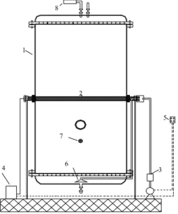
A schematic diagram of the pilot-scale rotation

reactor is showed in Figure 3. The reactor was

designed to accelerate the composting process by

optimizing temperature and air flow, to verify the

results of simulation model. The modes of aeration

studied were up flow through PVC tubing filled gas

chamber below a fine mesh screen near the bottom of

the reactor. Solid wastes temperature sensors were used for temperature measurements. The leachate of the system would be captured and recycled through the chamber rotation. This not only prevents the composts from drying out, but also prevents the removal of any bacteria, microorganisms that are essential to the process. Outlet vent installed an O

- H

S measuring apparatus: MD-520E instrument and CO

analyzer: LX-710.

1

2 8

5

4 6 3

7

Figure 3 Schematic diagram of experimental reactor. 1. main body; 2. axis; 3. gas flow meter; 4. electromotor; 5. control system; 6. air feedsystem; 7. temperature equipment; 8. gas analyzer.

The initial moisture content of the compost mixtures was around 60.0% (g H

O/g wet solids).

The organic substrate of raw materials was 35.0%.

Each pilot-scale composting tests was performed according to the conditions of simulation model. At the first time, the air flow was constant at 0.02 m

/（h·kg）. At the optimum condition, air flow was controlled and outlet oxygen concentration remains between 10 to 18%. This air flow served an additional service in keeping the reactor constantly aerated.

The solid wastes around 150 g were sampled to measure substrate concentration, moisture content, volatile solids at three points in the reactor. Moisture content was measured by oven drying at 101 for 24 h until a constant weight was obtained. Volatile solids content was determined by combusting samples at 550 for at least 6 h in a muffle furnace.

Total nitrogen content was determined using the

kjeldahl method while Carbon was determined using TOC analyzer.

Composite samples are processed for microbial count. The dilution plate is used to estimate the number of actinomycetes, bacteria and fungi in the samples. Mesophilic and thermophilic microbial strains are obtained by plating samples taken during composting progress in cultivating the plates at 30 and 60℃, respectively. Mesophiles and thermophiles are isolated and maintained on trytone soy agar (TSA) and peptone agar (PA), respectively.

Isolates are obtained by streaking out all the colonies of a spread plate within a sector containing 40 colonies. All isolates are tested for a number of properties on identical media, at 30 and 60℃.

A basal agar (BA) contained 0.1% peptone (Difco), 0.1% yeast extract (Difco) and 1.5% agar.

Test substrates were added to BA as follows: starch (0.5%), gelatine (1%), carboxymethyl cellulose (CMC, 1%), Chitin (swollen precipitated substrate, 30 ml/liter, and Tween 80 (1%) with CaCl

·2HO

(0.01).

3.2 Validations of Parameters

Coefficient and parameter values were estimated from experimental data and the literature (Hang, 1993). For example, For hydrocarbon compounds, heat quantity generated by unit organic in compost bulk, h

is 17.4 MJ/kg. For protein, h

is 23.4 MJ/kg. And for fat, h

is 39.3 MJ/kg.

According to the composition of solid waste used in pilot scale model, h

for organic substance in this study is selected as 17.6 MJ/kg. Potention thermal of water evaporation is 2.44 MJ/kg. Heat capacity of water, compost bulk and air,

,

and

, are 4.2, 2.1 and 2.1 kJ/(kg· ), respectively.

Under the condition of 55% water content, 60 , 0.02 m

/ （ h · kg ） air flow rate, microbial maximum specific grow rate is 0.18 (1/h);

=0.066;

is among the range of 0.02 to 0.07, in this study,

=0.04. For the pilot scale model, temperature of compost bulk, T

, is 60 and activate engery of compost bulk, E

, is 29 kJ/mol.

3.3 Validation Simulation model

Three scenarous are investigated with the

simulation model. The first simulation investigated

the interactions between substrate concentration,

microbial biomass growth, oxygen concentration

temperature and moisture content within the composter using a constant aeration rate. The second set of simulations using the roatation composter set- up, the aeration rate was controlled by the oxygen concentration in outlet exhust gas.

3.3.1 Predicted composter performance for a constant aeration rate

With developed dynamic simulation model, variations of compost indexes, such as compost bulk, organic components in compost bulk, mass of microorganisms, water content and temperature in the reactor and oxygen concentration in out air flow, are listed in Table 1 . The data of Table1 showed that most of compost indexes were decreased during the composting processeses except for temperature and mass of microorganisms. Temperature of compost bulk increased rapidly at the early stage, then kept stable. In the later stage of composting processeses, temperature declined gradually and the oxygen concentration in air outflow kept stable. It showed that function of air supply in this period was mainly cooling compost bulk. The mass of microorganisms kept increasing during composting processeses. The simulation results were consistent with the real experimental results (Table 1 and Figures 4 to 7) except that the error of temperature simulation was a little bit high. Reduction rates of solid waste were 60.36% and 50.08% through numerical model simulation and pilot scale experiments. Simulation result of organic substance degradation was 27.1%, while experimental result was 39.7%. Water content decrease of simulation was 37.13% and experimental result was 30.5%. The retention time of temperature above 55 was 156 hours for simulation result, however, it was 72 hours for experimental result. The reason of high temperature simulation error is perhaps the heat loss due to incomplete insulative reactor.

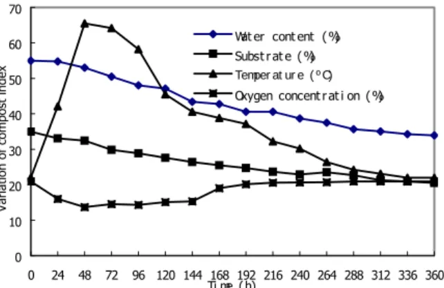
3.3.2 The aeration rate was controlled by the oxygen concentration in exhust gas

The simulation result of variations of compost indexes, are listed in Table 2. With developed dynamic simulation model, Air flow was adjusted so that outlet oxygen concentration in the exhaust gas remained a proper range to optimize the aeration costly. When the oxygen concentration was controlled the range from 10% to 18%, At the same

conditions, the experimental results are shown in Figure 8.

Comparison among simulation and experimental results showed that the developed model could well simulate solid waste composting processes.

Therefore, it could be used to instruct the design of optimal operation. The developed model may be used to simulate the efficiency and cost of compost processes 5nder different operation conditions. In this study, tHe air supply approach was adjusted and the developed model was then used to simulate the compost efficiency. It was identified, when composting pRocesses was on the way of iNtermittent operation, startinG air supply when oxygen concentration in air outflow lower than 10%

and stopping air supply wheN oxygen concentration higher than 18%, composting processes was very cost-effective. With this condition, running pilot scale experiment results in consistent reduction rate of organic substance (Figure 8). At the same time, oxygen supply was reduced 40% so that the cost of system operation was saved greatly. Thus, it is necessary to optimize the aeration mode to enhance the degradation rate of composting process and reduce air flow.

3.4 Sensitivity analysis

A simple sensitivity analysis was performed to

evaluate the relative importance of selected model

parameters. The parameter values examined were

maximum specific growth rate μ

, half velocity

constants for both degradable substrate ( K

) and

oxygen ( K

), yield coefficient ( Y ), initial biomass

concentration (X

), initial moisture content (W0) and

temperature (Temp0). These parameters were run in

the simulation program and all other parameters were

set at their default values. Then each parameter was

decreased to 60%, 40% and 25% of its default value

and then increased by 20%, 40% and 60% of its

default value over a 10-day simulation period. As

each parameter was varied, all other parameters were

maintained at their default values. All parameter

values used are shown in Table 3. Results from this

analysis are shown graphically in Figures 10 and

Figures 11.

Table 1. Simulation results with developed model Time

(h)

Total weight of compost bulk (kg)

Substrate (%)

Microbial (%)

Water

content (%) T (ºC) O

concentration in out flow (%)

0 100.00 35.00 1.00 55.00 22.0 20.90 24 97.65 33.94 1.97 54.87 53.88 17.79 48 88.73 33.34 4.18 52.34 67.54 14.77 72 79.64 33.10 6.68 48.92 67.57 15.08 96 71.28 32.74 9.58 45.05 67.15 15.53 120 63.85 32.23 12.86 40.81 66.45 16.04 144 57.44 31.53 16.44 36.36 65.47 16.59 168 52.09 30.60 20.22 31.90 64.12 17.15 192 47.76 29.47 24.00 27.69 62.25 17.72 216 44.40 28.18 27.57 23.97 59.35 18.37 240 42.36 27.21 30.07 21.47 47.53 19.64 264 41.39 26.62 31.39 20.25 37.23 20.19 288 40.80 26.23 32.23 19.48 31.85 20.40 312 40.35 25.93 22.89 18.88 29.08 20.51 336 39.97 25.69 33.44 18.35 27.37 20.58 360 39.64 25.51 33.91 17.87 26.11 20.64

0 10 20 30 40 50 60

0 48 96 144 192 240 288 336

Time (h)

Water content (%)

Experimental results Simulation results

0 10 20 30 40

0 48 96 144 192 240 288 336 Time (h)

Subs trate concentration Experimental results

Simulation results

Figure 4. Comparison of simulation and experimental Figure 5. Comparison of simulation and experimental results of water content results of substrate concentration

0 10 20 30 40 50 60 70 80

0 48 96 144 192 240 288 336 Time (h)

Temperature (ºC) Experimental results

Simulation results

0 5 10 15 20 25

0 48 96 144 192 240 288 336 Time (h)

Oxygen concentration (%)

Experimental results Simulation results

Figure 6. Comparison of simulation and experimental Figure 7. Comparison of simulation and experimental

results of temperature results of oxygen concentration

Table 2. Simulation results under designed operation condition Time (h) Total weight of

compost bulk (kg)

Substrate (%)

Microbial (%)

Air supply time (h)

Oxygen concentration (%)

0 105 33.33 0.95 0 20.90

24 102.67 32.34 1.85 12.90 14.67 48 93.30 31.65 4.0 36.90 14.94 72 83.44 31.43 6.45 60.90 15.22 96 74.35 31.11 9.33 84.90 15.64 120 66.25 30.63 12.61 108.90 16.13 144 59.24 29.95 16.25 132.90 16.65 168 53.37 19.03 20.15 156.90 17.19 192 48.62 27.87 24.12 180.90 17.73 216 44.91 26.53 27.93 195.90 7.36 240 42.60 25.46 30.70 200.90 15.80 264 41.51 24.79 32.18 203.70 15.84 288 40.84 24.33 33.14 205.51 10.38 312 40.33 23.97 33.88 207.00 28.65 336 39.91 26.69 34.52 208.10 10.90 360 39.53 23.45 35.07 209.20 12.92

Table 3. Parameter values used in sensitivity analysis

Change in Parameter analysis

Parameter Unit Percentage

-60 -40 -20 Default 20 40 60

S0 % 140 210 280 350 420 490 560 W0 % 220 330 440 550 660 770 880 Temp0 ℃ 8.8 13.2 17.6 22 26.4 30.8 35.2

X0 g/kg 4 6 8 10 12 14 16

μ

_h

_0.072 0.108 0.144 0.18 0.216 0.252 0.288

Kc g/kg 9.6 14.4 19.2 24 28.8 33.6 38.4

K

kg/m

0.017 0.0264 0.0528 0.066 0.0792 0.0924 0.1484

Y

kgx/kgs 0.2 0.3 0.4 0.5 0.6 0.75 0.9

0 10 20 30 40 50 60 70

0 24 48 72 96 120 144 168 192 216 240 264 288 312 336 360 Ti me (h)

Variation of compost index

Wat er cont ent (%) Subst r at e (%) Temper at ur e ( º C) Oxygen concent r at i on (%)

Figure 8. Experimental results under designed operation

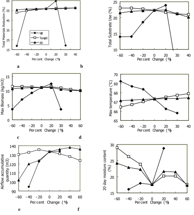
The output values examined were the total material reduction (kg), the total percent reduction in readily degradable substrate (ΔS, %) during the 10- day simulation, the maximum biomass concentration at any time (X

). The maximum compost temperature (T

, ℃ ) at any time, air flow quantity and moisture content during the 10 day simulation. In Figure 10 and Figure 11 the effects of changes in each parameter value on these four outputs are shown. For instance as varied from 0.072 to 0.288h

, X

increased from 6.721 to10.141 (kg/m

).

The sensitivity analysis demonstrated that several factors in the process (oxygen, biomass concentration, temperature, and moisture) interacted to control the rates of reactions. So, the interpretation of the results was not always straight forward because of these multiple interactions. For example, as Y

increased, fairly large increases in X

corresponding decrease in T

, (Figures 10c and 10d). As μ

increased and K

decreased, T

(Figure 10 d) increased; however, X

(Figure 10 c) and dS/dt (Figure 10b) have little changed. The slightly higher rates of substrate degradation at the increased μ

values were terminated much earlier due to low moisture levels. The decreased sensitivity of these outputs was due to limits placed on the growth process by the oxygen concentration, FAS, moisture and temperatures. Even more pronounced interactions were observed in the effect of increased μ

or Y

on the total reduction in substrate (Figure 10b). The maximum total substrate degradation (22.6%) occurred at the values of μ

=0.18h

and Y

=0.6.

As μ

decreased from its default value by 60%, a decrease in X of only 50.2% occurred because growth was inhibited somewhat by reduced oxygen levels, higher temperature and reduction of moisture.

Similarly, a decrease in the maximum rate of substrates gradation was observed, but it was decreased by only 6.75%. The higher temperature when μ

was decreased 60% (68.2 vs. 60.1 ℃ ) caused more rapid drying.

Changes in Kc or Ko had very little effect on the Total materials reduction of composting (Figure 10a), total substrate reduction (Figure 10b), maximum biomass (Figure 10c) and maximum compost temperatures (Figure 10d). Again, the air flow quantity and 10-day moisture content were regulated by changes in substrate and temperature levels.

Higher values of Kc and Ko or lower values in slightly effect composting processes.

Changes in the initial biomass concentrations (Xo) and initial temperature had extremely small effects (Figures 10a through 11f) on the magnitudes of the output values examined (less than 2%);

however, to different values of Xo, the times at which the maximum values were achieved shifted. For example, the maximum compost temperature occurred at 108 h for Xo=0.004 kg/m

and at 60 h for Xo=0.01 kg/m

.

Changing the initial moisture content (W0) from 22% to 71.5 resulted in major changes in all output variables except maximum temperature which only decreased from 69.2℃ to 65.8℃ (Figure 110 d).

However, the maximum temperature occurs in 240 h.

The effect of initial moisture content on the

composting processes is shown in more detail in

Figures 10f. Slighter high moisture content than

default provided more optimal conditions (Figures

11f) during the time periods when rapid composting

was occurring, but when it comes over 66%, the rate

of substrate degradation decrease. Particularly, when

moisture content is more than 71.5%, the composting

processes are impossible. As W0 decreased from its

default value by 60%, the total substrate use and the

X

are 2.123% and 0.0365 kg/m

, respectively. This

moisture depletion caused the durations of these

higher rates to be shorter and the total substrate

degradation was lower.

15 25 35 45 55 65

- 60 - 40 - 20 0 20 40 60

Per cent Change ( %)

Total Materials Reduction (%)

μmax Kc KO Yx/ s

10 15 20 25

- 60 - 40 - 20 0 20 40 60

Per c ent Change ( %)

Total Substrate Use (%)

μmax Kc KO Yx / s

a b

2 6 10 14

- 60 - 40 - 20 0 20 40 60

Per cent Change (%) Max temperature (℃)

60 63 66 69 72 75

- 60 - 40 - 20 0 20 40 60

Max temperature (℃)

c d

65 75 85 95 105 115 125

- 60 - 40 - 20 0 20 40 60

Per cent Change ( %)

Airflow accumulative quantity (m3)

10 20 30 40 50

- 60 - 40 - 20 0 20 40 60

Per cent Change (%)

20 day moisture content (%)

e f

Figure 10. Sensitivity analysis showing predicted model outputs as the indicated parameters ( μ

^, K

^, K

^, Y

^{) altered}

from –60% to +60% of its default value. (a) Total materials reduction. (b) Total substrate use. (c) Maximum biomass

concentration. (d) Maximum temperature. (e) Air flow accumulative quantity. (f) Moisture content profile.

15 25 35 45 55 65

- 60 - 40 - 20 0 20 30 40

Per cent Change ( %)

Total Materials Reduction (%)

W0 Temp0 X0

10 15 20 25

- 60 - 40 - 20 0 20 30 40

Per cent Change ( %)

Total Substrate Use (%)

a b

0 5 10 15

- 60 - 40 - 20 0 20 30 40 60 Per cent Change ( %)

Max Biomass (kg/m3)

65 66 67 68 69 70

- 60 - 40 - 20 0 20 30 40

Per cent Change ( %)

M ax temper at ur e ( ) ℃

c d

90 100 110 120 130 140

- 60 - 40 - 20 0 20 40 60 Per cent Change ( %) Air flo w accu m ulativ e quantity (m3)

15 20 25 30

- 60 - 40 - 20 0 20 40 60

Per cent Change ( %) 20 day moisture content (%)

e f

Figure 11. Sensitivity analysis showing predicted model outputs as the indicated parameters(W0, Temp0, X0) altered from –60%

to +60% of its default value. (a) Total materials reduction. (b) Total substrate use. (c) Maximum biomass concentration. (d)

Maximum temperature. (e) Air flow accumulative quantity. (f) Moisture content profile.

4. Conclusions

In this study, a dynamic model was developed to simulate composting processes of solid waste based on the thermodynamics and kinetics of microbial growth. The model provided an excellent vehicle for explaining and demonstrating the complex interactions which occur in the composting processes. Variations of compost indexes, such as substrate degradation, temperature fluctuations, moisture exchanges, and oxygen concentration were simulated for a readily composted input mixture. The model could be used to optimize operational parameters. For example, it was used to develop different aeration regimes through controlling the oxygen concentration in exhaust air to optimize the composting processes and reduce the air flow.

Another component should be controlled is the initial moisture content, the effect of initial moisture content on the composting processes was significant.

If the initial moisture content was too high or too low, it would reduce the rate of substrate degradation. Particularly, when moisture content was more than 71.5% or lower than 33% the composting processes was impossible. The simulation result was consistent with results of pilot scale experiment. It was found that function of air supply in the later stage was mainly cooling compost bulk. Developed numerical model could be used to help identifying more cost-effective operation condition for composting processes. Adjusting operation conditions through changing key factors, optimal operation condition could be determined through comparing the results of numerical simulation. In this study, the optimal way of air supply was designed with the help of numerical model. Real experimental results showed that it could reduce 79.61% of oxygen supply with the same compost efficiency. Therefore, developed numerical model is of great significance to instruct the operation of real composting processes and reduce the operation cost.

Acknowledgement:

Foundation item: The National “973” of China (No.: 2002C410800-07) and The National “973” of China (No.: 2002CB412302).

Correspondence to:

Beidou Xi, Zimin Wei

Chinese Research Academy of Environmental Sciences

Beijing 100012, China

Telephone: 01186-10-8491-3946 Cellular phone: 01186-130-3103-8107;

01186-131-4100-9271

Emails: [email protected]; [email protected] References

[1] Vallini G, Pera A, Valdrighi M, Cecchi F. Process constraints in source-collected vegetable waste composting. Wat Sci Technol 1993;28(2):229- 36.

[2] Huang JS, Wang CH, Jih CG. Empirical Model and Kinetic Behavior Thermophilic Composting of Vegetable Waste. Journal of Environmental Engineering 2000; 126(11):1019-25.

[3] Miller F. Composting of municipal solid waste and its components. Microbiology of Solid Waste. CRC Press: 1996:116-45.

[4] Hammelers H. A Theoretical Model of Composting Kinetics. Science and Engineering of Composting. The Ohio State University.

1993:37-58.

[5] Haug RT. Development of Simulation Models, In: The Practical Handbook of Compost Engineering, Lewis Publishers 1993:385-436.

[6] Hamoda MF, Abu HA, Newham J. Evaluation of municipal solid waste composting kinetics.

Resources, Conservation and Recycling 1988;

23(1): 209-23.

[7] Mohee R, White RK. Simulation Model for Composting Cellulosic (Bagasse) Substrates.

Compost Science & Utilization 1998; 6(2): 82- 92.

[8] Agamuthu P. Kinetic Evaluation of Composting of Agricultural Wastes. Environmental Technology 2000; 21(1):185-92.

[9] Quazi H, Bari AK, Tao G. Kinetic analysis of forced aeration composting—Reaction rates and temperature. Waste manage Res 2000; 18:303- 12.

[10] Stombaugh DP, Nokes SE. Development of a Biologically Based Aerobic Composting Simulation Model. Transactions of ASAE 1996;

39(1):239-50.

[11] Keener H, Marugg C, Hansen RC, Hotink H.

Optimizing the Efficiency of the Composting

processes. Science and Engineering of Composting 1993; The Ohio State University:

59-94.

[12] Wang HT, Li YS. Simulation model of dynamic aerobic compost and the application. China

Environmental Science 2001 (in Chinese);21(3): 240-4.

[13]

.

.

, 1993:4.

11/5/2009