R ESEARCH I NSTITUTEFOR M ATHEMATICAL S CIENCESKYOTOUNIVERSITY,Kyoto,Japan ByMasanobuINUBUSHIJanuary2013 CovariantLyapunovAnalysisofNavier-StokesTurbulence RIMS-1770

(1)

RIMS-1770

Covariant Lyapunov Analysis of Navier-Stokes Turbulence

By

Masanobu INUBUSHI

January 2013

R _ESEARCH I NSTITUTE FOR M ATHEMATICAL S _CIENCES

KYOTO UNIVERSITY, Kyoto, Japan

(2)

Covariant Lyapunov Analysis of Navier-Stokes Turbulence

Masanobu Inubushi

Research Institute for Mathematical Sciences,

Kyoto University

(3)

(4)

—Abstract—

Turbulence is a ‘disordered’ state of fluid motion but shows robust and universal statistical properties including Kolmogorov -5/3 law and Prandtl logarithmic law, which we can observe in laboratory experiments, numerical experiments, and observations. It is important for a wide range of sciences and engineering to understand mechanisms of turbulence which produce such robust statistical properties. However, at present, our understanding is far from complete.

Turbulence can be interpreted as a chaotic dynamical system and this point of view is expected to provide a broader perspective to understand turbulence. In this thesis, we focus our attention on an orbital instability which is one of the important properties of chaos. Particularly, we employ covariant Lyapunov analysis recently developed by Ginelli et al. (2007), which gives Lyapunov vectors associated with Lyapunov exponents.

First of all, we study the orbital instability of chaotic Kolmogorov flows.

Kolmogorov flow is a fluid flow on a two-dimensional torus governed by the incompressible Navier-Stokes equation and its bifurcation and stability have been under intense study (Okamoto, 1998). We study relations between hyperbolic property and physical property of the chaotic Kolmogorov flow.

Hyperbolicity is one of the fundamental properties of dynamical systems related to the orbital instability. Recently, hyperbolicity of the chaotic Kol- mogorov flow was studied by employing the covariant Lyapunov analysis, where the hyperbolic-nonhyperbolic transition was observed as the Reynolds number is increased (Inubushiet al., 2012). Here, our interest lies in relations between the hyperbolic properties and physical properties of fluid motions.

We study correlation decay of vorticity at several Reynolds numbers across the hyperbolic-nonhyperbolic transition point. We find that an oscillation in time-correlation function vanishes at the transition point. Furthermore, examining the energy dissipation rate and the angle between the stable and unstable manifolds θ, we show that the angle θ tends to be small when the energy dissipation rate is large in a statistical sense.

Next, we study the orbital instability of Couette turbulence. Couette turbulence is fluid turbulence between moving walls governed by the three- dimensional incompressible Navier-Stokes equation, often being studied with interests in the transition to turbulence and coherent structures in turbulence. Particularly we examine regeneration cycles which are important phenomenon observed in a wide variety of wall-turbulence including the Couette turbulence. The regeneration cycle is consisting of breakdown (in the first half period of the cycle) and reformation (in the last half period of the cy-

i

(5)

cle) ofstreaks which are well-known coherent structures. Here, a goal of this study is to characterize the regeneration cycle with the orbital instability by employing the covariant Lyapunov analysis. Firstly, we present the Lya- punov spectrum of the Couette turbulence, and we discuss the dimension of unstable manifold, the dimension of the attractor, and the Kolmogorov-Sinai entropy. To see the orbital instability of the regeneration cycle in more detail, we study the local Lyapunov exponents and the associated Lyapunov modes. With these quantities, we find that (1) at the breakdown of the streaks, the Lyapunov modes indicate asinuous instability which makes the streaks meander, (2) when the streamwise vorticity is highly localized, the local Lyapunov exponents appear to attain their maxima in the regeneration cycle, and (3) the local Lyapunov exponents decrease rapidly and become negative after the localization of the streamwise vorticity. These results suggest that the ‘most unstable’ instability during the regeneration cycle is the instability associated with the strong localization of the streamwise vorticity rather than the sinuous instability. Also, instabilities are found only in a very early stage of the cycle and after that there are no exponential instability at all. Finally, we reconsider the regeneration cycle from the viewpoint of the orbital instability. There, we argue the physical mechanisms of the streak meandering (breakdown) and the localization of the streamwise vorticity, which can be characterized by the Lyapunov modes. Then, examining the evolution equation of the modal energy, we discuss the mechanism of the streak reformation which closes the cycle. We find that the streaks are reformed by interactions with mean flows and furthermore the energy is injected into a ‘streak mode’ from the mean flows almostconstantlythroughout the regeneration cycle. There, a natural question arises : what controls the development of the streaks (i.e. the regeneration cycle)? Finding an answer to the question, we study the energy flows in the system during the regeneration cycle in detail and detect an interaction between the streak mode and a ‘meandering mode’ that controls the regeneration cycle.

ii

(6)

Chapter 1 Introduction

Turbulence as a chaotic dynamical system.— Is dynamical system the- ory useful to understand turbulence? Turbulence is a ‘disordered’ state of fluid motion but shows robust and universal statistical properties including Kolmogorov -5/3 law in energy spectra of isotropic homogeneous turbulence and the Prandtl logarithmic law in mean velocity profiles of wall turbulence.

We can observe such statistical properties in laboratory experiments, numerical experiments, and observations. These properties appear to be independent of the details of the system such as the way of excitation of turbulence and the boundary condition [1, 2]. It is important to understand turbulence mechanisms of producing such robust statistical properties for a wide range of sciences and engineering field. However, at present, our understanding is far from complete.

Dynamical system theory gives general concepts to study asymptotic states of a dynamical system, and gives tools to quantify the degree of ‘dis- order’ of the states [3, 4]. From this point of view, the theory is expected to provide a broader perspective to understand turbulence, where we consider turbulence as a state point on a chaotic attractor in a phase space and gain new insights into turbulence by using such concepts and tools as bifurcations, periodic orbits, Lyapunov exponents and so on [5]. At the same time, understanding of the turbulence at this viewpoint may provide an important bridge between fluid system and high-dimensional dynamical systems in other fields.

One of the pioneer works on turbulence from a mathematical standpoint was done by Ruelle and Takens [6]. They considered definition of turbulence by discussing bifurcations of a (quasi-)periodic orbit and showed¹that

1See Proposition (9.2) in [6].

1

(9)

1 Introduction

a chaotic attractor appears by adding an arbitrary small perturbation to a quasi-periodic system². Then, they proposed an idea that turbulence can be described in terms of a chaotic attractor rather than a quasi-periodic attractor with a large number of (rationally independent) frequencies as proposed by Landau [10]³. This idea has been verified both experimentally and numerically in many studies. For instance, Gollub and Swinney [12] examined bifurcations in a rotating fluid in detail by employing power spectra, and demonstrated that the onset of turbulence is consistent not with the Lan- dau picture but with Ruelle and Takens picture. Nowadays, most of the researchers have reached a consensus, following Ruelle and Takens idea, and there are many studies on turbulence considering it as a chaotic attractor⁴.

Chaos is often characterized by the following concepts: denseness of un- stable periodic orbits(UPOs) andorbital instability(cf. Devaney’s definition of chaos⁵). Considering turbulence as chaos, invariant solutions including UPOs and orbital instability of the Navier-Stoles equation are important, and they have been studied numerically with an increase in computing power.

Invariant solutions within turbulence.— A number of the invariant so- lutions of the Navier-Stoles equation, numerically discovered recently, such as steady solutions, traveling wave solutions, and periodic solutions, are useful for understanding bifurcations of solutions, global structures of the phase space, and statistical properties of turbulence. Okamoto [17] studied bifurcations ofKolmogorov flow (see chapter 5 in [18] and chapter 2 in this thesis) and considered singular-limit flows in association with turbulence. Schneider

2In addition to this scenario (Ruelle-Takens scenario), we now know that there are some scenarios leading to chaotic attractor (route to chaos) : Feigenbaum scenariothrough period doubling andPomeau-Manneville scenariothrough intermittency. See Eckmann [7]

and Ott [8] for details. Inubushiet al. [9] studied Kolmogorov flow and found that chaotic fluid motion appears with Pomeau-Manneville scenario, in particularType-I intermittency (see appendix A.1).

3See [11] for a description of view of turbulence at that time.

4In this thesis, we refer tofluidturbulence as ‘turbulence’, although sometimes the term

‘turbulence’ is used to describe disordered state found in general dynamical systems, including coupled map lattices, Kuramoto-Sivashinsky equation, complex Ginzburg-Landau equation, and so on [13].

5Roughly speaking, dynamical systemf on an invariant set V is called to bechaotic in Devaney’s senseif (1)f istransitive, (2) periodic points off are dense inV, and (3)f has sensitive dependence on initial condition (see p.50 in [14]). However, now it is known that these conditions are not isolated, i.e. the condition (3) is followed by the conditions (1) and (2) [15]. Here we refer to the condition (3) as orbital instability. See§2.3 in Oono [16] for the definition of chaos from an interesting perspective.

2

(10)

et al. [19] found spatially localized solutions in Couette flow (see chapter 3) and argued a ‘snakes-and-ladders’ structure in their bifurcation diagram.

On global structures in the phase space, invariant solutions play important roles in understanding of transition to shear turbulence, where a stable manifold of an invariant solution (‘lower branch solution’ or a ‘gentle’ UPO) is considered as a separatrix between basin of attraction of laminar flow and that of turbulent flow (see Itano and Toh [21], Waleﬀe [20], and Kawahara [22]). Halcrow et al. [23] showed several heteroclinic connections between these invariant solutions and discussed changes of coherent structures along the heteroclinic connections. In a relation with statistical properties of turbulence, a concept and a method of a cycle expansion are significant, by which we can calculate statistical quantities of turbulence in principle if the attractor of the turbulence is hyperbolic (see chapter 2) and we have some knowledge of the attractor (e.g. Floquet exponents of UPOs embedded in the attractor. see Cvitanovic [24]). Although the cycle expansion provides the statistical quantities by an infinite weighted sum of information of UPOs, Kawahara and Kida [25] found that statistical quantities such as a mean velocity profile and root mean square velocity profiles can be well approxi- mated by a single UPO with low period embedded in Couette turbulence⁶. van Veen and Kawahara [26] recently computed homoclinic orbit to a time- periodic edge state (the gentle UPO) in Couette turbulence. They showed that the homoclinic orbit is related tobursting eventsin both spatiotemporal and statistical senses. Kato and Yamada [27] found a UPO in a shell model⁷ of three-dimensional turbulence (GOY model⁸), which reproduces not only the Kolmogorov -5/3 law but also interimttency observed in turbulence, and suggested that averaged properties on the attractor can be described by the UPO as far as lower-order quantities are concerned. These findings on the invariant solutions make us realize fundamental questions and oﬀer intrigu- ing hints for understanding of turbulence.

Orbital instability.— In contrast to invariant solutions of the Navier- Stokes equation, which is actively investigated as seen above and reviewed by Kawahara [29], chaotic properties of the Navier-Stokes turbulence itself (e.g.

6Why can a single UPO with low period give an good approximation to the statistical properties of the turbulence? Saiki and Yamada [28] argued this fundamental and intrigu- ing question by studying the statistical properties of more than 1000 UPOs and those of chaotic orbits in low-dimensional dynamical systems.

7They referred to this UPO as ‘intermittency solution’ [27].

8Gledzer-Ohkitani-Yamada model.

3

(11)

1 Introduction

Fig. 1.1: Illustration of an orbit in a phase space. Red (u⁽¹⁾₀ ) and blue (u^(m)₀ ) arrows denote Lyapunov vectors associated with the Lyapunov exponents λ₁(>0) and λ_m(<0) respectively. u⁽¹⁾₀ indicates unstable direction andu^(m)₀ indicates stable direction along the orbit.

the properties of the orbital instability) appear to be attracting less interest in spite of their importance. One of the fundamental quantities characteriz- ing the orbital instability isLyapunov(orcharacteristic)exponentsand their associated vectors (Lyapunov vectors). Considering a dynamical system defined by a map f : R^m → R^m (equipped with some norm || · ||), we write time evolution of a state point in a phase space x_n ∈R^m as x_n+1 = f(x_n).

An infinitesimal perturbation vectors (tangent vectors)u^(j)n (j = 1,2,· · ·, m) added to the state point x_n evolves, obeying the linearized equation:

u^(j)_n =Df_x_n₋₁u^(j)_n₋₁, (1.1) where Df_x_n is am×m Jacobian matrix. By using the chain rule of diﬀer- entiation, we write

u^(j)_n =Df_x_n₋₁u^(j)_n₋₁ =Df_x_n₋₁ Df_x_n₋₂· · ·Df_x₀u^(j)₀ =Dfⁿu^(j)₀ . (1.2) whereu^(j)₀ denotes an initial perturbation vector at an initial pointx₀. Then j-th Lyapunov exponent λ_j (λ₁ ≥λ₂ ≥ · · · ≥λ_m) is defined as

±λ_j = lim

n→±∞

1

|n|ln||Dfⁿu^(j)₀ ||, (1.3) and the associatedj-th Lyapunov vector at x_n is defined asu^(j)n . The set of Lyapunov exponents{λ₁, λ₂,· · · , λ_m}are referred to as Lyapunov spectrum.

4

(12)

In physical systems, such as a system describing turbulence, the Lyapunov exponents are considered to be independent of the choice of the initial point⁹ x0. The Lyapunov exponent λj quantifies an exponential growth (or decay) rate of the norm of the perturbation added to the orbit, and correspondingly, the Lyapunov vector points to the direction of the perturbation vector (see Fig.1.1). Once we obtain the Lyapunov exponents λj (j = 1,2,· · ·, m), we can calculate also attractor dimension D_L (Lyapunov dimension) through Kaplan-Yorke formula : D_L=K+_|_λ ¹

K+1|

∑K

j=1λ_j whereK is the largest in- teger such that ∑K

j=1λ_j ≥0 and Kolmogorov-Sinai (or metric)entropy h_KS through Pesin identity : h_KS =∑

λj>0λ_j [5, 8]. To Study the instability of the dynamics in more detail, local (or finite-time) Lyapunov exponents are sometimes useful, which is defined as ˜λ_j(k, s) = _|_k¹_|ln||Df^ku^(j)s ||. The local Lyapunov exponents ˜λj(k, s) depend on state pointxs and ‘local mean time’

k, which captures local orbital instabilities (see chapter 3). A numerical algorithm to compute Lyapunov exponents was first proposed by Shimada and Nagashima [30], who employed Gram-Schmidt orthogonalization of the tangent vectors. The orthogonalized tangent vectors obtained by the algorithm are referred to asGram-Schmidt vectors. Note that the Gram-Schmidt vectors diﬀer from Lyapunov vectors in general except the Lyapunov vector associated with the largest Lyapunov exponent λ₁.

Characterization of turbulene with orbital instability.— Using this algorithm for GOY model, Yamada and Ohkitani [32] obtained an asymptotic scaling law of the Lyapunov spectrum by using the Kolmogorov scaling theory. Karimi and Paul [33] characterized Rayleigh-B´enard convection with the Lyapunov vector associated with the largest Lyapunov exponent.

They demonstrated statistically that a transition from ‘boundary-dominated’

dynamics to ‘bulk-dominated’ dynamics occurs when the system size is increased. Keefe et al. [34] calculated the Lyapunov spectrum of turbulent Poiseuille flow at Reynolds number Re = 3200 and found that the dimension of the attractor is ‘dauntingly high’, estimating the attractor dimension D_L ≃ 780 by using Lyapunov spectra. Recently, Nikitin [35] studied the

9Given some ergodic invariant measure ρ, the limit (1.3) exists for ρ-almost allx₀ in a great generality (multiplicative ergodic theorem). See §9 in Ruelle [5] for more precise statements. Recently, Ott and Yorke [31] constructed two dynamical systems on R² and showed that in these dynamical systems the Lyapunov exponent does not exist when we choosex0in the basin that is not on the attractor. However, as mentioned in their paper, the flows defined by these dynamical systems are not generic in the space of smooth flows onR²and far from physical systems.

5

(13)

1 Introduction

largest Lyapunov exponent λ₁ of turbulent flows in a circular tube and in a plane channel over a range of Reynolds number 4000 ≤Re≤ 10700 (140 ≤ Reτ ≤ 320) and showed that the largest Lyapunov exponent normalized by the ‘wall time scale’¹⁰ appears to be a constant value independent of the Reynolds number and the type of the wall turbulence. While these findings on the statistical quantities are important for understanding of the chaotic properties of the turbulence, it is also expected to use the Lyapunov analysis to elucidate the dynamics of turbulence (e.g. regeneration cycle of wall turbulence. See chapter 3). However it remains out of reach.

Covariant Lyapunov analysis.— As well as Lyapunov exponents, Lya- punov vectors may possess essential information of turbulent dynamics since they point to unstable directions of an orbit which indicate instability mechanisms to generate the turbulence. Although the conventional Lyapunov analysis employing numerical algorithms based on the method of the Shimada and Nagashima [30] gives the proper Lyapunov exponents, it only gives the Gram-Schmidt vectors instead of the Lyapunov vectors. It is diﬃcult to find the physical meaning of the Gram-Schmidt vectors, since these vectors (i) depend on a definition of an inner product and (ii) are diﬀerent from those in the backward time evolution (i.e. they are not invariant under time reversal).

Both of these properties (i) and (ii) are not consistent with the definition of the Lyapunov vectors. On the other hand, in a finite dimensional smooth dynamical system, the Lyapunov vectors are the tangent vectors which do not depend on the definition of the inner product and give the same Lyapunov exponents except for their signs in the forward or backward time evolution.

The Lyapunov vectors are bases of the local stable and unstable tangent spaces according to the signs of the Lyapunov exponents. Recently Ginelliet al. [36] proposed an algorithm, which is called covariantLyapunov analysis, to obtain the Lyapunov vectors. The covariant Lyapunov analysis employs the conventional Lyapunov analysis as a first part of the algorithm, where the Gram-Schmidt vectors are computed in the forward time evolution. We then compute the tangent space dynamics confined to suitable subspaces in backward time evolution by using the stored Gram-Schmidt vectors. In the backward time evolution, the vectors in the subspaces converge generically to the Lyapunov vectors after suﬃciently long time. Besides the covariant Lya- punov analysis, Wolfe et al. [37] proposed another computational method to calculate the Lyapunov vectors, what is called characteristic Lyapunov

10The time scale tτ which is determined by the near-wall physics (i.e. defined by the

‘wall friction’ velocityuτ and lengthlτ astτ=lτ/uτ). See chapter 3 for more details.

6

(14)

vectors¹¹. These vectors, which have been applied to some chaotic systems such as coupled-map lattices [38], are also independent of the inner product and covariant under the tangent space dynamics (for the detailed comparison between these methods, see Kuptsov et al. [39]).

Thanks for the development of these numerical algorithms, the Lyapunov vectors have been used to study both conservative and dissipative dynamical systems. Yang and Radons [40] calculated the Lyapunov vectors of coupled maps lattice. They examined hydrodynamic Lyapunov modes (HLMs)¹² , what they call, in relation to non-equilibrium statistical mechanics, which supports their hypothesis : a certain hyperbolic property¹³ is crucial for ob- serving the HLMs. Employing the covariant Lyapunov vectors, Yang et al. [42] found an approach to study inertial manifolds which are finite- dimensional manifolds attracting trajectories exponentially [43]. While the inertial manifold is considered to be an important concept, it has been dif- ficult to construct the inertial manifold of the partial diﬀerential equation in a concrete way. Yang et al. [42] divided Lyapunov vectors into ‘physical’

and ‘isolated’ modes in the case of the Kuramoto-Sivashinsky equation and complex Ginzburg-Landau equation and then speculated that there is some relation between the number of the physical mode and the dimension of the inertial manifold. These findings have a great importance since the existence of the inertial manifold and its dimension would justify numerical simulations of the dissipative partial diﬀerential equations with finite resolution¹⁴. Hyperbolicity and relation to physical property.— As mentioned above, Lyapunov vectors are tangent to stable and unstable manifolds of an invariant set, and we can study hyperbolicity of the invariant set by the Lyapunov vectors. Hyperbolicity is one of the fundamental properties of dynamical systems. A dynamical system is called to be hyperbolic if the tangent space of the phase space can be decomposed into stable and unstable sub-

11Ginelli et al. [36] called the covariant Lyapunov vectors by simply ‘the Lyapunov vectors’. In this thesis, we refer to the covariant (or characteristic) Lyapunov vector as simply ‘Lyapunov vector’ in distinction from Gram-Schmidt vector.

12Hydrodynamic Lyapunov modes are long-wavelength Lyapunov modes associated with near-zero Lyapunov exponents, which is expected to give a novel insight into a many-body problem. See Yang and Radons [40] for details.

13The hyperbolic property they studied in [40] is ‘partial domination of the Oseledec splitting’ with respect to subspaces associated with near-zero Lyapunov exponents.

14Futhermore, Yang and Radons [44] proposed a method to compute the dimension and to study the geometry of the inertial manifolds of spatially extended dissipative dynamical systems by using Gram-Schmidt vectors.

7

(15)

1 Introduction

spaces, i.e., the stable and unstable manifolds intersect at nonzero angles.

When a dynamical system possesses the hyperbolic property, its theoretical analysis is easier in general compared with nonhyperbolic cases. Also, hyperbolicity is deeply connected to the structural stability of the dynamical systems [45]. Measurement of the angle between the local stable and the local unstable manifolds along the solution orbit shows whether the attractor is hyperbolic or not, and how far the hyperbolic attractor is from the nonhyperbolic state. (sometimes referred to as degree of hyperbolicity). Although there are some algorithms to compute global stable and unstable manifolds of steady solutions or periodic solutions and these algorithms have been applied to the solutions of fluid system [46, 47], it is still diﬃcult to compute the stable and unstable manifolds of chaotic solutions. Saiki and Kobayashi [48] calculated angles between stable and unstable manifolds of Lorenz attractor by using the covariant Lyapunov analysis and identified a hyperbolic parameter region¹⁵. Also, by the covariant Lyapunov analysis, Kuptsov et al. [50] identified the hyperbolic parameter regions of the coupled Ginzburg- Landau equations. They found that the system becomes nonhyperbolic at the same parameter value where the third Lyapunov exponent becomes positive, and furthermore, argued that the system exhibits an extensive spatiotemporal chaos after the hyperbolic-nonhyperbolic transition. Artuso et al. [51]

showed that a fixed point of some two-dimensional area-preserving map loses its hyperbolicity at certain control parameter values, which is associated with changes of the asymptotic decay rate of time correlation: when the system is hyperbolic the time correlation decays exponentially, and when the system is nonhyperbolic the time correlation decays algebraically. These findings are interesting in the way that they suggest that the change of the hyperbolic property has a physical interpretation as well. Considering these findings, It is natural to ask if the hyperbolic properties of physical systems such as fluids governed by the Navier-Stokes equation are related to their physical propertes. One of the goals of this thesis is to obtain the answer to this question.

What we study in this thesis.—In this thesis, we study orbital instability of turbulence through the covariant Lyapunov analysis. Here we focus our attention on the orbital instability of the chaotic Kolmogorov flow and the Couette turbulence. Kolmogorov flow is a fluid flow on the two-dimensional

15Recently they also studied manifold structures of UPOs embedded in the Lorenz attractor, and found that the angles between stable and unstable manifolds of them are related to appearance of periodic windows in a bifurcation diagram [49].

8

(16)

torus governed by the Navier-Stokes equation and its bifurcation and stability have been under intense study as it has been considered as a simplest example which contains essential elements of the Navier-Stokes flows. Cou- ette turbulence is fluid turbulence between moving walls governed by the three-dimensional Navier-Stokes equation, and is sometimes referred to as a

‘canonical example’ of the wall-turbulence, often being studied with interests in the transition to turbulence and coherent structures in turbulence.

Recently, hyperbolicity of the chaotic Kolmogorov flow was studied by employing the covariant Lyapunov analysis, where the hyperbolic-nonhyperbolic transition was observed (§IV of [52]). In§2 of this thesis, we review the result of hyperbolic-nonhyperbolic transition appearing in the chaotic Kolmogorov flows. Here, our interest lies in relations between the hyperbolic properties and such physical properties of fluid motions as time correlation of the vorticity and the energy dissipation rate. First, we study the correlation decay of the vorticity at several Reynolds numbers across the hyperbolic- nonhyperbolic transition point. We find that the hyperbolic-nonhyperbolic transition is reflected in the qualitative change of the long-time correlation functions : before the transition the time-correlation function decays exponentially with oscillation and after the transition it decays purely exponential (i.e. the oscillation in time-correlation function vanishes at the transition point). Furthermore, examining the energy dissipation rate and the angle between the stable and unstable manifolds θ, we report that the angleθ tends to be small when the energy dissipation rate is large in a statistical sense.

In §3, we study the orbital instability of the Couette turbulence. Par- ticularly we examine regeneration cycles observed in a wide variety of wall- turbulence including the Couette turbulence. The regeneration cycle is an important phenomenon consisting of breakdown (in the first half period of the cycle) and reformation (in the last half period of the cycle) of streaks which are well-known coherent structures (see §3 for a detailed description).

The goal of this chapter is to characterize the regeneration cycle with the orbital instability by employing the covariant Lyapunov analysis.

First in§3, we present the Lyapunov spectrum of the Couette turbulence.

From the Lyapunov spectrum, we obtain the dimension of the unstable manifold, the dimension of the attractor, and the Kolmogorov-Sinai entropy. Then we compare these information on the chaotic attractor with results reported in previous studies on the Floquet exponents of UPOs embedded in the turbulent attractor [69, 70], the normalized maximum Lyapunov exponent of the wall turbulence at the high Reynolds number [35], the attractor dimension of the Poiseuille turbulence [34], and the dimension of the dynamical system

9

(17)

1 Introduction

models of the regeneration cycle [62].

Next, to see the orbital instability of the regeneration cycle in more detail, we study the local Lyapunov exponents and the associated Lyapunov modes.

With these quantities, we find that (1) at the breakdown of the streaks, the Lyapunov modes indicate a sinuous instability which makes the streaks meander, (2) when the streamwise vorticity is highly localized, the local Lyapunov exponents appear to attain their maxima in the regeneration cycle, and (3) the local Lyapunov exponents decrease rapidly and become negative after the localization of the streamwise vorticity (i.e. they appear to be positive only in a very early stage of the cycle). These results suggest that the ‘most unstable’ instability during the regeneration cycle is the instability associated with strong localization of the streamwise vorticity rather than the sinuous instability. Also, instabilities are found only in a very early stage of the cycle and after that there are no exponential instability at all.

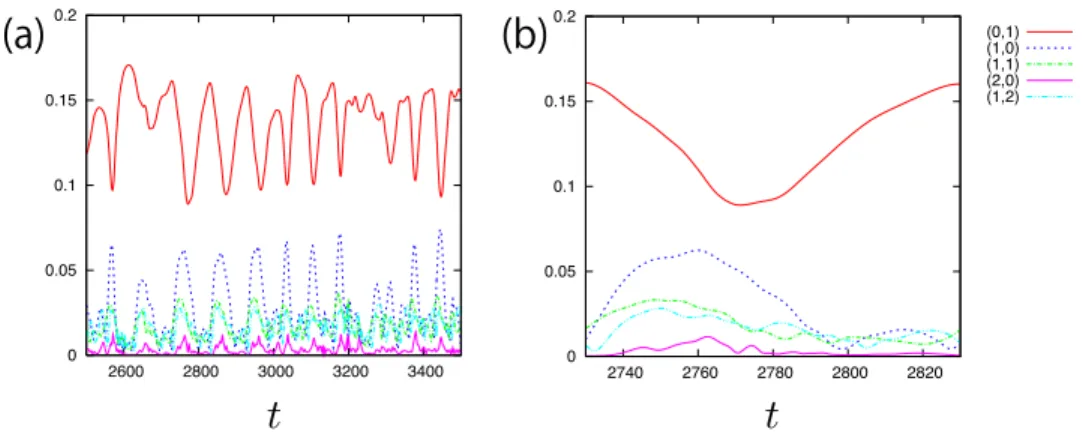
In the final part of§3, we reconsider the regeneration cycle from the viewpoint of the orbital instability. There, we argue the physical mechanisms of the streak meandering (breakdown) and the localization of the streamwise vorticity, which can be characterized by the Lyapunov modes. Particularly, we conclude that the localization of the streamwise vorticity is caused by the vortex stretching and propose a detailed mechanisms of it. Then, examining the evolution equation of the modal energy, we discuss the mechanism of the streak reformation which closes the cycle. We find that the streaks are reformed by interactions with mean flows and furthermore the energy is injected into the ‘streak mode’ from the mean flows almostconstantlythroughout the regeneration cycle. In other words, the interactions with mean flows reform the streaks throughout the cycle steadily. There, a natural question arises : what controls the development of the streaks (i.e. the regeneration cycle)?

Finding an answer to the question, we study the energy flows in the system during the regeneration cycle in detail and detect the interaction between the streak mode and a ‘meandering mode’ that controls the regeneration cycle. The regeneration cycle in the wall turbulence is important not only for science but also for engineering, thus there are a great deal of research on the regeneration cycle. However, as far as we know, the orbital instability picture of the regeneration cycle described above has been never proposed.

Finally, in §4 we summarize the whole thesis and discuss future issues.

10

(18)

Chapter 2 Relations between hyperbolic properties and physical

properties of chaotic Kolmogorov flow

2.1 Introduciton

Hyperbolicity is one of fundamental properties of dynamical system as mentioned in§1. Despite the importance of hyperbolic property, there are few ex- amples of concrete dynamical systems whose hyperbolic properties are known in a rigorous manner. At present, we know the some exact results of hyperbolic properties of low-dimensional dynamical systems at best such as real H´enon family studied by Arai [53]. However recently, the covariant Lyapunov analysis gave us a new way to estimate hyperbolicity of even high-dimensional dynamical systems (Ginelli et al. [36]).

Fluid turbulence is often viewed as a typical example of chaos appearing in high-dimensional dynamical systems and hence hyperbolic property of turbulence can be important in understanding of it from the viewpoint of dynamical system. As a first step to obtain knowledge of the hyperbolic property of turbulence, Inubushi et al. [52] studied the degree of hyperbolicity of the Kolmogorov flows. This fluid system was proposed by Kolmogorov to study the stability and bifurcation of the solutions of the Navier-Stokes equation [17] and the route to chaos [54]. As shown in Fig.2.1, the Lyapunov exponents increase with the Reynolds number and the Kolmogorov flows be-

11

(19)

2 Relations between hyperbolic properties and physical properties of chaotic Kolmogorov flow

come chaotic (λ₁ >0)¹ at the Reynolds number²R/R_cr ≃18.2, under which the fluid motion is quasi-periodic (λ₁ = λ₂ = 0) (see §III in [52] and §2.3 for details). Employing the covariant Lyapunov analysis, Inubushi et al.

showed probability density functions of the angle between the local stable and unstable manifolds along the solution orbit and they found hyperbolic- nonhyperbolic transition at a certain Reynolds number (see §IV in [52] and

§2.4).

The hyperbolic-nonhyperbolic transition may be expected to influence long-time statistical property of the flow. In order to study the physical properties of chaotic Kolmogorov flows, we here focus our attention on two physical quantities; the time-correlation of the vorticity and the enstrophy (the energy dissipation rate). This chapter is organized as follows. In §2.2, we describe Kolmogorov flow system and numerical method. Then in §2.3, we summarize briefly chaotic solution of Kolmogorov flows whose behavior is studied in later sections. We show the main result in this chapter in§2.4:

relations between the hyperbolic properties and the physical properties of the system. §2.4.1 and §2.4.2 are devoted respectively to descriptions of relations between the degree of hyperbolicity and time correlation functions and relations between the angleθ and enstrophy. Finally, we summarize and discuss the obtained results in§2.5.

2.2 Kolmogorov flow system and numerical method

Kolmogorov flows are fluid flows governed by the two-dimensional incompressible Navier-Stokes equation and the vorticity equation which we solve numerically is

∂_tζ+u· ∇ζ = 1 R

(

∆ζ−n³cosny )

, (2.1)

where u = u(x, y, t) = (u, v) is the velocity, ζ = ζ(x, y, t) = ∂_xv−∂_yu the vorticity,R the Reynolds number,nthe wave number of the external forcing.

Because of this simple form of external forcing, Kolmogorov flow has two kinds of symmetries ; if ζ(x, y) is a solution of the vorticity equation (2.1),

1In the Kolmogorov flow system, Pomeau-Manneville scenario leads to chaotic attractor with Type-I intermittency. See appendix A.1 and Inubushiet al. [9]

2Rcr is critical Reynolds number of “trivial solution”. See later sections for details.

12

(20)

2.2 Kolmogorov flow system and numerical method

-0.06 -0.05 -0.04 -0.03 -0.02 -0.01 0 0.01 0.02 0.03

18 19 20 21 22 23 24 25

18.2

3.4 4.0 5.0 5.4

18 19 20 21 22 2324 25

Fig. 2.1: Lyapunov exponents λ_i (i = 1,2,· · ·5, λ₁ ≥ λ₂ ≥ · · · ≥ λ₅), the horizontal axis is Reynolds number R/R_cr (18.0 ≤ R/R_cr ≤ 25.0). Inset ; Lyapunov dimension D_L. It is found that 3.5 ≲ D_L ≲ 5.5 in this range of the Reynolds number

then G^jζ(x, y) (j = 1,2,· · · ,2n−1 , G^j = G| ◦ · · · ◦{z G}

j

) and T_αζ(x, y) (α ∈ [0,2π)) are also a solution, where

Gζ(x, y) = −ζ(−x, y−^π_n) (2.2) T_αζ(x, y) =ζ(x−α, y). (2.3) Roughly speaking, G represents a discrete “shift” by π/n in y direction and T_α represents a continuous “shift” by α in xdirection.

The governing equation (1) possesses a steady solutionζ =−ncosny (so- called the trivial solution) and we denote byR_cr(= n√

2) the critical Reynolds number beyond which the trivial solution becomes linearly unstable in the domain x ∈ [0,2π) (periodic) and y ∈ (−∞,∞). Iudovich showed that for the forcing wavenumbern = 1, the trivial solution is globally and asymptot- ically stable [55]. Here we focus our attention on the chaotic solution of the Kolmogorov flows, in the case of the forcing wavenumber n = 2.

Direct numerical simulations of the vorticity equation (1) are performed by means of the standard 2/3 dealiased spectral method on the periodic domainT² = [0,2π)×[0,2π) where the number of the grid points is 24×24,

(21)

-0.2 0 0.2

-0.2 0 0.2 -0.2

0 0.2

-0.2 0 0.2

I 1 ,

ζ0

R 1 ,

ζ0 ζ0^R,1 ζ0^R,1

I 1 ,

ζ0 ζ0^I,1

Fig. 2.2: The projection of the solution orbit onto (ζ_0,1^R , ζ_0,1^I ) plane at (a) R/R_cr = 18.0, (b) R/R_cr = 20.0, (c) R/R_cr = 24.0 (1.0×10⁴ ≤ t ≤ 3.0×10⁴). Only at (a) R/R_cr = 18.0, there are four solution orbits arising from four diﬀerent initial conditions.

and truncated wave numbers were 7×7 as ζ(x, y, t) =

∑K,L

k=−K, l=−L

ζ_k,l(t)e^i(kx+ly) (2.4)

where K =L = 7. A state of the Kolmogorov flows is represented by a set of the Fourier coeﬃcients

(ζ_−K,−L^R (t), ζ_−K,−L^I (t),· · · , ζ_K,L^R (t), ζ_K,L^I (t))∈R^N^′

(N^′ = 2(2K+ 1)(2L+ 1)), (2.5)

where ζ_k,l^R(t) and ζ_k,l^I (t) (−K ≤ k ≤ K,−L ≤ l ≤ L) are respectively the real and imaginary parts of the complex Fourier coeﬃcients ζk,l(t) satisfying the Hermitian symmetry, ζ_k,l(t) = ζ₋^∗_k₋_l(t) where ∗ denotes the complex conjugate. In addition,ζ₀₀vanishes, and therefore the dimension of the phase space (degrees of freedom) of the truncated system is N = (2K + 1)(2L+ 1)− 1 = 224. We used the library for spectral transform ISPACK [66], its Fortran90 wrapper library SPMODEL library [67] and the subroutine of LAPACK. For time integration, we used the 4th order Runge-Kutta method with the time step ∆t= 5.0×10⁻³. For drawing the figures, the products of the Dennou Ruby project [68] and gnuplot were used.

2.3 Chaotic behavior of Kolmogorov flow

In this section, we summarize briefly the chaotic solution of Kolmogorov flows making use of the Lyapunov analysis. The time integration of the

(22)

2.3 Chaotic behavior of Kolmogorov flow vorticity equation (2.1) shows that the flows are quasi-periodic at R/R_cr ≲ 18.2 and chaotic at R/R_cr ≳18.2. To clarify the instability of the flows, we calculate the Lyapunov exponents λi (i = 1,2,· · ·5, λ1 ≥ λ2 ≥ · · · ≥ λ5) of Kolmogorov flow at different Reynolds numbers (Fig.2.1). Also, to illustrate the solution orbit in the phase space, in Fig.2.2 we show a projection of the solution orbit in the phase space onto (ζ_0,1^R , ζ_0,1Î ) plane at R/Rcr = (a) 18.0, (b) 20.0, (c) 24.0 (1.0×10⁴ ≤ t ≤ 3.0×10⁴). We use four different initial conditions ζ_k,l^(j)(j = 0,1,2,3)

ζ_k,l^(j)= {

0 (k=l = 0),

ζ₀₁^(j)δ0,kδ1,l+ (1 +i)_k¹⁰2+l⁻³² (otherwise), (2.6) where ζ_0,1^(j)= 0.2(1 +i)e^π²^ij atR/R_cr = 18.0.

AtR/R_cr = 18.0, there are four stable quasi-periodic solutions (λ₁ =λ₂ = 0 > λi(i = 3,4,· · ·N) Fig.2.2 (a)) due to the symmetry (2) of the system : G rotates the phase of Fourier componentζ_0,1 byπ/2 [rad], i.e. Gζ_0,1 =iζ_0,1. The quasi-periodic solution is composed of two plus/minus rapidly oscillating vortices (the period of oscillating motion T1 ≃ 35) slowly traveling to x direction (the period of traveling motion T₂ ≃ 1241), which is confirmed by a power spectrum (see Fig.2.11). The two zero Lyapunov exponents λ₁ = λ2 = 0 (Fig.2.1) are due to the property of the autonomous system and the translational symmetry in x direction of this system corresponding to T_α in the equation (2.3).

The Lyapunov exponents increase monotonically with Reynolds number (Fig.2.1). And atR/R_cr ≳18.2, the quasi-periodic solutions become unstable (λ₁ >0) and merge into a large chaotic attractor composed of the four (unstable) quasi-periodic solutions and their connecting orbits (Fig.2.2 (b)). This route to chaos observed in the Kolmogorov flow can be characterized by so- called Type-I intermittency (see appendix A.1) [9]. The chaotic solution then wanders around the unstable quasi-periodic solutions and “jumps” between them intermittently. The energy (E = ¹₂||u||²_L²) and the energy dissipation rate (ε = 2Q/R where Q= ¹₂||ζ||²_L² is the enstrophy) also undergo intermit- tent bursts simultaneously with the “jumps” (Fig.2.3). The time series of the energy E and the energy dissipation rateεare quite similar, bursting almost simultaneously. The energy injected by the external forcing dissipates so quickly, which implies the absence of the inertial subrange and the energy cas- cade in wavenumber space, in contrast with fully developed turbulence. Actu- ally, the flow fields is in a state of not spatiotemporal but temporal chaos, consisting of two plus/minus large vortices oscillating chaotically in time. The

(23)

0.003 0.004 0.005 0.006 0.007 0.008

10000 15000 20000 25000 30000

0.05 0.06 0.07 0.08 0.09

10000 15000 20000 25000 30000

Fig. 2.3: Time series of the energy E and the energy dissipation rate ε at R/Rcr = 20.0 (1.0×10⁴ ≤t≤3.0×10⁴).

Lyapunov dimension D_L=K+ _|_λ ¹

K+1|

∑K

i=1λ_i (K = max{m|∑m

j=1λ_j ≥0}) (inset of Fig.2.1) is found to be rather small (3.5 ≲ D_L ≲ 5.5) in harmony with the observation of the temporal chaos. At R/R_cr ≃ 23.0, the 2nd positive Lyapunov exponent emerges, and at higher Reynolds number the solution orbit appears less trapped by the unstable quasi-periodic solutions (Fig.2.2 (c) at R/R_cr = 24.0).

2.4 Covariant Lyapunov analysis of chaotic Kolmogorov flow

In this section, we review the covariant Lyapunov analysis of chaotic Kol- mogorov flow, in particular the study on degree of hyperbolicity³.

Localization of the Lyapunov vector in physical space and wavenumber space is often related to characteristic physical properties of a chaotic behavior. In the “spiral defect” chaos in Rayleigh-Benard convection, the spatially localized pattern of the first Lyapunov vector is associated with the creation and annihilation of the defects [56], while in a shell model of turbulence (GOY model), an asymptotic scaling law of the Lyapunov spectrum can be obtained by using the localization property of Lyapunov vectors in wave number space

3Published in Inubushiet al. [52].

(24)

2.4 Covariant Lyapunov analysis of chaotic Kolmogorov flow

(a) (b) (c)

x

y ^0.64

-0.693 0

1.8 0 -1.8

0.135 0 -0.135

0 π 2π

x

0 π 2π

x

0 π 2π

π

0 2π

π

0 2π

y ^π

0 2π

+ y - -

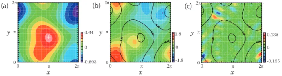
Fig. 2.4: Stream functions at t= 1.0×10⁴ of (a) solution, Lyapunov vectors corresponding to (b)λ1and (c)λ200 atR/Rcr = 20.0. The contours in (b),(c) shows the stream function of the solution.

and Kolmogorov scaling theory [32].

Now we can calculate the whole of the Lyapunov vectors by the covariant Lyapunov analysis for the chaotic Kolmogorov flows. Fig.2.4 (a) is the snapshot of the stream function of the chaotic solution as stated above and Fig.2.4 (b) and (c) are the stream functions of the Lyapunov vectors corresponding respectively to the Lyapunov exponentλ1 andλ200 att = 1.0×10⁴, R/R_cr = 20.0. The norm of the perturbation by the Lyapunov vector in Fig.2.4 (b) grows nearly exponentially (λ₁ >0), while that in Fig.2.4 (c) decays nearly exponentially (λ200 <0). The spatial scale of the first Lyapunov vector is nearly the same as the solution, and that of the 200th Lyapunov vector is smaller. This implies that the Lyapunov vectors corresponding to λ1 (λ200) is composed of low (high) wavenumber Fourier modes. Then we define the time averaged energy spectra E(j, n) =E(j, n, t) of the j-th Lya- punov vector q^(j) where the overline denotes time average ¯· = _T¹ ∫_T

0 · dt, n = 1,2, ...,√

K²+L² the total Fourier wavenumber, and E(j, n, t) = 1

2∆_n

∑

n²≤k²+l²<(n+1)²

(|uˆ^(j)_k,l(t)|²+|vˆ^(j)_k,l(t)|²) .

Here (ˆu^(j)_k,l,vˆ^(j)_k,l) is the complex Fourier coeﬃcient of the velocity u^(j) = (u^(j)(x, y), v^(j)(x, y)) of the j-th Lyapunov vector q^(j) and ∆_n = π{(n + 1)² −n²}. We use T = 16.0×10⁴ for the time average and the Lyapunov vector q^(j) is normalized with respect to the energy norm as ¹₂||u^(j)||²_L² =

∑

nE(j, n, t)∆_n= 1. Fig.2.5 (a) shows log₁₀E(j, n) at R/R_cr = 20.0, where we confirmed that the qualitative properties do not depend on the Reynolds

(25)

0 50 100 150 200

1e-10 1e-09 1e-08 1e-07 1e-06 1e-05 0.0001 0.001 0.01 0.1

1 10

j=1 j=50 j=100 j=150 j=200

1 2 3 4 5 6 7 8 9

Fig. 2.5: (color online) (a) Energy spectra of Lyapunov vectors. The horizontal axis is the Lyapunov indicesj, the vertical axis is Fourier wavenumber n and the contour is the energy spectra log₁₀E(j, n) at R/R_cr = 20.0. (b) the cross section of (a) fixed Lyapunov indices (j = 1,50,100,150,200).

number (20.0 ≤ R/R_cr ≤ 24.0). The energy spectra E(j, n) for fixed Lya- punov indexj = 1,50,100,150,200 are also shown in Fig.2.5 (b). It is found that the peak of energy spectrum shifts toward higher wavenumber with the increase of Lyapunov index. This is consistent with the dominance of small structures in Fig.2.4(c). This localization of Lyapunov vectors at high wavenumbers is in accidence with the correspondence between the Lyapunov exponents and the viscous dissipation, λ ∼ −_R¹k², where k is the localized wavenumber of the Lyapunov vector [32].

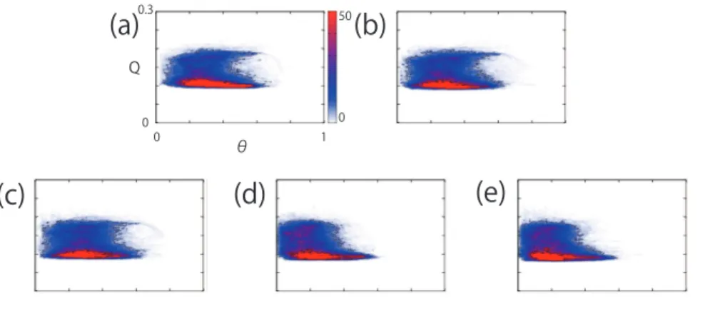
In order to evaluate the hyperbolicity of the chaotic motion, we calculate the probability density functions of the angle θ between the local stable and unstable manifolds along the solution orbit. Fig.2.6 is the closeup around zero angle (0[rad] ≤ θ ≤ 0.1[rad]) of the PDF P(θ) at R/R_cr = 20.0,21.0,22.0,23.0,24.0 from top to bottom with error bars (see APPENDIX B in [52] for details).

We find that at the small Reynolds number (R/R_cr ≃20.0) the distribution of the angle vanishes at zero angle (P(0) = 0), which indicates that the attractor is hyperbolic. However, as the Reynolds number is increased, the anglesθ has more chance to take smaller values and the distribution extends toward the zero angle. And at a certain Reynolds number (R/Rcr ≃ 23.0) the distribution of the angles is observed to reach the zero angle (P(0)>0), which implies that the attractor becomes non-hyperbolic. It should be re- marked that R/Rcr ≃ 23.0 is near the Reynolds number where the 2nd

(26)

2.4 Covariant Lyapunov analysis of chaotic Kolmogorov flow

0 0.05 0.1 [rad]

R/Rcr=20.0

R/Rcr=21.0

R/Rcr=22.0

R/Rcr=23.0

R/Rcr=24.0 0.001

0.01 0.1 1 10

Fig. 2.6: (color online) Close-up (0[rad] ≤θ ≤0.1[rad]) of the PDF P(θ) at R/R_cr = 20.0,21.0,22.0,23.0,24.0 from top to bottom (linear-log plot) with error bars (see APPENDIX B in [52] for details).

(27)

0.01 0.1 1

0 200 400 600 800 1000 1200 1400 0.9

1

0 10

R/Rcr=20.0 R/Rcr=21.0

R/Rcr=22.0 R/Rcr=23.0

R/Rcr=24.0 5

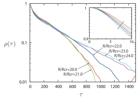
Fig. 2.7: The time-correlation function ρ(τ) (linear-log plot). Inset is an close-up of the time-correlation function in 0≤ τ ≤10 (the arrow indicates increase of the Reynolds number).

Lyapunov exponent become positive (Fig.2.1).

2.5 Relations between hyperbolic properties and physical properties of chaotic Kol- mogorov flow

We expect that the hyperbolic-nonhyperbolic transition aﬀects long-time statistical property of the flow, as mentioned in §2.1. In this section, the main part of this chapter, we focus our attention on two physical quantities; the time-correlation of the vorticity and the enstrophy (the energy dissipation rate).

2.5.1 Hyperbolicity and correlation fuction

The time-correlation function of the vorticity ζ(t) =ζ(x^′, y^′, t) is defined as

˜

ρ(τ) = ζ(t)ζ(t−τ)−ζ². (2.7)

(28)

2.5 Relations between hyperbolic properties and physical properties of chaotic Kolmogorov flow

-0.0005 0 0.0005 0.001 0.0015 0.002

19 20 21 22 23 24 25

Fig. 2.8: Dependence of the fitting parameter ω on the Reynolds number (19.0≤R/Rcr ≤25.0)

Fig.2.7 shows the normalized time-correlation function ρ(τ) =⟨ρ(τ˜ )⟩/⟨ρ(0)˜ ⟩ at (x^′, y^′) = (π/4, π/4) where⟨·⟩ denotes ensemble average over M diﬀerent initial conditions. In the inset of the figure a close-up of the correlation function ρ(τ) in the short-time range (0 ≤τ ≤10) is presented. Each initial condition is the trivial solution with a random perturbation as

ζ_k,l⁽ⁱ⁾ = {

0 (k=l = 0)

−ⁿ₂δ_k,0(δ_l,n+δ_l,₋_n) +P⁽ⁱ⁾ (otherwise),

where P⁽ⁱ⁾ = r⁽ⁱ⁾(1 + i)_k¹⁰2+l⁻³² and r⁽ⁱ⁾(r = 1,2,· · ·M) is uniform random numbers in an interval [0,1). We use T = 2.0× 10⁵ and M = 30 and confirmed that the qualitative properties of correlation do not depend on the T, M and the observation point (x^′, y^′).

In a short-time range (0≤τ ≤10), chaotic Kolmogorov flows exhibit an algebraic decay (ρ(τ)∼1−cτ², c ≃0.0012) of the time-correlation function independently of the Reynolds number. However, in long-time range (τ ≳ 100) the decay of the time-correlation changes at R/R_cr ≃ 22.0 ; the time- correlation function at R/R_cr = 20.0,21.0 decays super-exponentially, and changes its sign, while the time-correlation function at R/Rcr = 23.0,24.0 has an exponential tail ρ(τ)∼e⁻^{τ /T}.

We employ the least-square method to fit the time-correlation function with ρ(τ) =ae⁻^{τ /T} cosωτ via three fitting parameters (a, T, ω) in long-time