複雑環境下における物体検出のための背景モデリング

(1)

九州大学学術情報リポジトリ

Kyushu University Institutional Repository

複雑環境下における物体検出のための背景モデリング

吉永, 諭史

https://doi.org/10.15017/1441255

出版情報：Kyushu University, 2013, 博士（工学）, 課程博士バージョン：

権利関係：Fulltext available.

(2)

Background Modeling for Object Detection in Complex Situations

Satoshi Yoshinaga

Department of Advanced Information Technology

Graduate School of Information Science and Electrical Engineering Kyushu University

January 2014

(3)

(4)

List of Figures

2.1 Examples of typical background changes with the results of the background subtraction employing a fixed background image: (a) shows a case of the il- lumination changes, where the sunlight gets into the background. (b) shows a case of the dynamic changes, where trees are swaying in the wind. . . . 8 2.2 Calculation of a local binary pattern . . . . 9 2.3 Generation of a radial reach correlation . . . . 10 2.4 Problems related to the appearance and disappearance of stationary objects . . 14 2.5 Problems related to overlaps between moving foreground objects and stationary

foreground objects . . . . 16

3.1 Proposed background model based on Statistical Local Difference Pattern: Lo-

cal Difference (LD) is a local feature, and is defined by the difference between

a target pixel and a neighboring pixel. LD is modeled using a Gaussian mixture

model (GMM) to represent its distribution, making it a statistical local feature

called the Statistical Local Difference (SLD). The proposed model defines the

Statistical Local Difference Pattern (SLDP) using several SLDs for the back-

ground model (this figure shows an example with six SLDs). . . . 18

(9)

LIST OF FIGURES

3.2 Adaptivities of the proposed model to background fluctuation: (a) shows the case of illumination changing suddenly (e.g. when sunlight is blocked by clouds).

SLDP can adapt to illumination changes. This is because LD has the ability to tolerate the effects of illumination changes which affect the target pixel value in proportion with others. (b) shows the case of texture changing periodically (e.g. the effect of movement of tree or grass). GMMs can adapt to these kinds of dynamic changes, since they can learn the variety of background hypotheses. 19 3.3 The datasets for evaluation . . . . 23 3.4 Examples of foreground detection results using a PETS dataset (scene1) . . . . 25 3.5 Foreground detection results using Wallflower dataset . . . . 28 4.1 Similarity in the intensity changes among pixels: A set of pixels, each pixel of

which are geographically and chromatically close to each other, shows similar intensity changes against illumination changes. . . . 32 4.2 Example of a result of the pixel clustering using a K-means algorithm ( K =

100): The clustering result at least shows that each cluster contains the pixels belonging to the same part of the scene context (e.g., grass, road, sky, and walls of the buildings). . . . 34 4.3 Examples of foreground detection results using synthetic videos of the BMC

database . . . . 42 4.4 Examples of the difference in the effect on the background between illumination

changes and the fog . . . . 43 4.5 Examples of foreground detection results using real videos of the BMC database 46 5.1 Object-level multi-layered background modeling framework: This is the scene

that two pedestrians pass in front of a bus stop, where a yellow bus stops after a

blue bus has stopped there. . . . 51

(10)

LIST OF FIGURES

5.2 The overall processing flow of the object-level multi-layered background mod- eling: First, in the multi-layered object detection, both moving foreground ob- jects and stationary objects are detected. Next, in the object-layer update, the appearance and disappearance of stationary objects are detected, and the corre- sponding object-layers are added to/deleted from the multi-layered background model. Finally, in the multi-layered background model update, for each pixel, a background model belonging to the most recently added object-layer is updated using an input image. . . . 52 5.3 The detailed process of multi-layered object detection using the object-level

multi-layered background model: For each pixel, all the object-layers are ex- amined to see which layer is matched to the pixel in the order of L

^max

to L

¹

. . 55 5.4 The details of the object-layer update according to the foreground object state

analysis: This process creates and adds new object-layers for each stationary object, which is an object continuously “staying” at one position, to the multi- layered background model. . . . . 57 5.5 Foreground object state analysis: (a) and (b) correspond to the states where

a bus is “moving” and “staying,” respectively. The overlap images visualize the similarities of blobs between two consecutive images, and the similarity increases in proportion to the overlap ratio. In a case where a ratio of deeply- colored area exceeds a threshold, a corresponding blob is determined as “stay- ing.” . . . . 58 5.6 The details of the object-layer update according to the stationary object state

analysis: This process detects the disappearance of a stationary objects and

delete their corresponding object-layers from the object-level multi-layered back-

ground model. . . . . 60

(11)

LIST OF FIGURES

5.7 Examples of stationary stationary object state analysis: (a) visualizes the object- level multi-layered background model at time t . (b) and (c) show the examples where the states of a stationary object, i.e., the yellow bus, are “still existing”

and “disappeared,” respectively. . . . . 61 5.8 The transition of pixel clusters of each object-layer: Red arrows show how the

pixel clusters of lower object-layers are divided for a new object-layer. Blue arrows show how the pixel clusters of an abandoned object-layers are merged into the lower object-layers. . . . . 62 5.9 Examples of multi-layered object detection in complex situations: White and

black pixels correspond moving foreground objects and the first object-layer, i.e., the initial background, respectively. Red and yellow pixels correspond to stationary objects. In cases of red pixels, they occlude only the initial back- ground. In contrast, in cases of yellow pixels, they occlude existing stationary objects in addition to the initial background. . . . . 65 5.10 Comparison of object detection in complex situations: The first row corre-

sponds to the scene of “bus stop morning.” The second and third rows cor- respond to the scene of “bus stop evening,” where the bus moves away (corre- sponding to the third row) after staying at the bus stop (corresponding to the second row). From the fourth to the last rows correspond to each view point of an intersection. . . . 68 A.1 Gaussian mixture model representation of a probability density function . . . . 85 B.1 Rectangular kernel used in the fast background modeling algorithm using kernel

density estimation: This figure shows an example with d = 1 in Eq.(B.1). . . . 89 B.2 Fast update mechanism of the background model based on kernel density esti-

mation . . . . 91

(12)

List of Tables

3.1 Object detection accuracy using PETS and LIMU datasets . . . . 24

3.2 Performance evaluation using Wallflower dataset . . . . 27

4.1 Evaluation results using 5 synthetic videos of “Street” for evaluation phase . . . 40

4.2 Evaluation results using 5 synthetic videos of “Rotary” for evaluation phase . . 41

4.3 Evaluation results using 9 real videos of the BMC database . . . . 45

5.1 Accuracy of object detection in complex situations . . . . 67

(13)

(14)

Chapter 1 Introduction

With the development of information technology, digital cameras are widely used in our life for various purposes. For example, surveillance cameras are installed in airports, stations, downtowns and other public places for security surveillance. Additionally, they are installed along most roads for traffic surveillance, and are installed in shopping malls for marketing research. Conventionally, to use them for various purposes described above, videos from those surveillance cameras had been monitored and analyzed only by human beings. However, in the now, the increase of the video surveillance cameras requires us to find methods and algorithms for dealing with the huge amount of information gathered every second. Therefore, to achieve automatic analysis of videos, computer vision, which aims at duplicating the abilities of human vision by electronically perceiving and understanding images, has been getting more and more attention recently.

In computer vision technologies, one of the most important research issues is object de-

tection which identifies foreground objects in a sense. This is because foreground objects in-

formation can be used in various applications, such as security, tracking, action recognition,

etc. In this thesis, the author proposes an on-line algorithm for detecting foreground objects

from image sequences captured by a static camera. Furthermore, the author proposes an object

detection framework to adapt to complex situations such as a bus stop, where pedestrians and

cars pass in front of a stopped bus. The rest of this chapter consists of the “Background of the

(15)

Chapter 1. Introduction

research,” “Aim of the research” and “structure of the thesis.”

1.1 Background of the research

Object detection allows to identify foreground objects in a sense and its detection results are used for various purposes. For example, in video surveillance applications such as home and office security systems, it is possible to raise an alarm when someone enters a restricted area based on the object detection. Object detection results can also be used to help observers mon- itor the security situation of monitoring area by emphasizing regions of foreground objects.

Furthermore, identification of foreground objects allows further (high-level) processing, which needs to identify foreground target objects in a scene. By estimating correspondence between objects in consecutive image frames, information of foreground objects can be used for tracking particular objects of interest. Additionally, features extracted from foreground object regions can be used for human action recognition and scene understanding.

As described above, object detection is used in various applications, and then, the more accurate detection techniques are required to improve the performance of these applications.

However, due to a wide range of variations in foreground objects, background changes, etc., it is difficult to accurately detect foreground objects. To detect foreground objects robustly against these factors, many object detection methods and algorithms have been proposed [1–4]. The paper [1] summarizes example-based object detection methods which detect foreground objects based on physical appearance defined by visual features such as Haar-like [5, 6] and Histogram of Oriented Gradients (HOG) [7–9] features. Most of these methods have used the cascade classifier structure together with ensemble learning methods, e.g., AdaBoost [10]. Then, in order to train weak classifiers, large amounts of training data is required for each category of foreground objects, such as pedestrians, cars, etc. Therefore, it is difficult to use these methods for surveillance in a new scene, because a lot of prior knowledge and training data suitable for the new scene are required.

Background subtraction, which removes a background image from an input image, enables

(16)

1.1 Background of the research

us to overcome this constraint. It enables us to detect foreground objects without any prior knowledge of them, and therefore, it is widely used for foreground object detection in prac- tical applications. However, when background subtraction is applied to outdoor surveillance, image sequences observed by the cameras often include not only foreground objects but also background changes, which are caused by lighting condition changes or the fluctuations in the scene. Therefore, many researchers have proposed various background modeling approaches to detect foreground objects robustly against background changes [2–4]. To cope with background changes caused by the fluctuations in the scene, such as swaying motion of tree branches, the previously observed intensity values are statistically modeled [11–14]. However, these statisti- cal approaches cannot adapt to lighting condition changes, where intensity values of each pixel are rapidly and significantly affected and then unseen intensity values are observed. To handle background change caused by lighting condition changes, some local features have been used for background modeling [15–19]. However, these local feature-based methods have difficulty handling background changes caused by the fluctuations in the scene, which affect the local features in the background significantly. To address these problems, hybrid background mod- els [20–22], which combine detection results of multiple different background models, have also been proposed. However, these methods mistakenly detect specific background regions, affected by lighting condition changes and the fluctuations in the scene at the same time. This is because these researches assume that either statistical or local feature-based models can always adapt to background changes correctly.

Furthermore, even though many background models have been proposed, the problem of background maintenance in complex situations, in which not only moving objects but also sta- tionary objects are observed, is still far from being completely solved. In a bus stop, for ex- ample, where pedestrians and cars pass in front of a stopped bus. In such situations, stationary objects, such as a stopped bus, should be detected as “foreground.” However, most conventional approaches have mistakenly treated such stationary foreground objects as parts of “background”

to detect the moving foreground objects passing in front of the stationary objects. Moreover,

such situations cause another problem when foreground objects move away after staying in one

(17)

Chapter 1. Introduction

position for a long time. Conventional methods falsely detect background regions uncovered by such foreground objects. This is because conventional background models have only one background layer and assume all the foreground objects keep moving.

Background subtraction using background models is an effective technique for object de- tection, because it allows to detect foreground objects without prior knowledge. However, as described above, there are still some problems with background models. Major problems in background modeling can be summarized as follows.

Problem 1: To detect foreground objects robustly against various background changes, back- ground models should be able to adapt to various background changes even when some regions are simultaneously affected by multiple different factors, such as the lighting con- ditions and fluctuations in the scene.

Problem 2: To correctly detect foreground objects in complex situations, such as a bus stop and a train platform, a new background modeling framework, which can detect stationary objects as well as moving objects, is required. Then, the moving foreground objects passing in front of the stationary objects need to be distinguished from stationary objects.

Additionally, when stationary foreground objects move away after staying in the same position for a long time, the framework needs to be able to treat the regions uncovered by such foreground objects as “background.”

1.2 Aim of the research

This thesis aims to develop an on-line background modeling framework, which can detect not only moving foreground objects but also stationary objects robustly against various background changes in complex situations. To achieve this goal, we have to consider the major problems in background modeling as discussed above.

To solve the problem 1, the author has proposed to employ a spatio-temporal information

by intrinsically integrating the methodologies of statistical and local feature-based approaches

(18)

1.3 Structure of the thesis

into a single framework. Then, the background model has properties of both statistical and local feature-based approaches. Therefore, the spatio-temporal background model can adapt to various background changes, even if some regions are affected by different types of background changes at the same time. In this thesis, the author proposes two types of spatio-temporal back- ground models suitable for outdoor surveillance

¹

. In the first type, the author defines a local feature using a difference between pixels which are close in pixel coordinate, and the temporal information of the local feature is modeled in a statistical framework. Then, because the prop- erties of the pixels cannot be considered, in the first type, the use of the spatial information is limited to define the local feature for adapting to lighting condition changes. To use the spatial information more efficiently, in the second type, by considering a set of pixels whose intensities change in a similar manner to each other, a region-level statistical information is used. In other words, by statistically modeling the relationship of intensity changes among the pixels, the sec- ond type can use the spatiality to adapt not only to lighting condition changes but also to the fluctuation in the scene.

To solve the problem 2, the author proposes a new background modeling framework, in which background models for each stationary object are hierarchically conserved in addition to one for the initial background. By applying this framework to the spatio-temporal back- ground model, we can detect both moving foreground and stationary foreground objects ro- bustly against various background changes.

1.3 Structure of the thesis

This thesis consists of Chapter 1 “Introduction,” Chapter 2 “Related works,” Chapter 3 “Back- ground model based on a statistical local difference pattern,” Chapter 4 “Background model using a spatio-temporal similarity of intensity changes,” Chapter 5 “Object-level multi-layered background modeling in complex situations” and Chapter 6 “Conclusion.” The outlines of each

1

The target scenes are mainly “long shot” scenes in the outdoors, and the proposed method is not intended for

“close-up shot” scenes in which a foreground object is very large.

(19)

Chapter 1. Introduction

chapter are as follows.

In Chapter 2, the merits and drawbacks of the conventional background models are dis- cussed. Additionally, the problems in the maintenance of background models, which are com- mon to most conventional background models, are discussed.

In Chapter 3, the author proposes a statistical local difference pattern (SLDP), by applying a statistical framework to a local feature, which is stable to lighting condition changes, defined based on the spatiality. Then, the SLDP has both properties of statistical and local feature-based approaches. In the experiments, the performance of object detection is evaluated and compared with conventional background modeling approaches.

In Chapter 4, the author proposes a new spatio-temporal background model based on a spatio-temporal similarity of intensity changes (StSIC). By considering a relationship among a set of particular pixels whose intensity changes are similar to each other, the StSIC allows the spatial information to be used to adapt not only to lighting condition changes but also to the fluctuation in the scene. In the experiments, the performance of object detection is evaluated and compared with the SLDP in addition to conventional background models.

In Chapter 5, the author proposes an object-level multi-layered background modeling frame- work for object detection in complex situations. In this framework, multiple background models are used to model the features of each stationary object, e.g., the visual appearance, and they are hierarchically conserved in addition to one for the initial background. In the experiments, the StSIC is introduced into this framework, and then the performance of object detection in com- plex situations is evaluated and compared with conventional background modeling approaches.

Finally in Chapter 6, the main contributions in the thesis are summarized, and the future

works are discussed.

(20)

Chapter 2 Related works

One of the fundamental problems in computer vision is detecting regions or objects of inter- est from an image sequence. Background subtraction, which removes a background image from an input image, is widely used for foreground object detection in practical applications because it enables us to detect foreground objects without any prior knowledge of the objects. However, when background subtraction is applied to outdoor surveillance, the “long shot” scenes of cam- eras often include not only foreground objects but also background changes related to lighting conditions or the fluctuations in the scenes because the cameras are often installed in high lo- cations to obtain a large field of view. In general, background changes that occur in outdoor scenes can be classified into two types: the one is caused by lighting condition changes, and the other is caused by the fluctuations in the scene. In this thesis, the author calls the former as “il- lumination changes” and the latter as “dynamic changes” as follows, and their typical examples are shown in Figure 2.1.

• Illumination changes – changes relating to lighting conditions such as the sun rising, setting, or being blocked by clouds (see Figure 2.1(a)),

• Dynamic changes – changes relating to the swaying motion of tree branches, leaves and

grasses, fleeting clouds, waves on water and so on (see Figure 2.1(b)).

(21)

Chapter 2. Related works

Subtraction result Ground truth

Input image Background image

(a) Illumination changes

Subtraction result Ground truth

Input image Background image

(b) Dynamic changes

Figure 2.1: Examples of typical background changes with the results of the background sub- traction employing a fixed background image: (a) shows a case of the illumination changes, where the sunlight gets into the background. (b) shows a case of the dynamic changes, where trees are swaying in the wind.

To detect foreground objects robustly against background changes, we have to be able to handle these background changes. Therefore, as reported in the survey papers [2–4], many researchers have proposed a lot of background modeling approaches. Based on the methodologies of back- ground modeling, we can categorize conventional background models into three main types:

local feature-based background models, statistical background models and hybrid background

models. Each approach has some of its own characteristics, which influence the results of ob-

ject detection. Therefore, in this chapter, these background modeling approaches are reviewed

in the following three sections. After that, the maintenance of background models, which are

common problems to most conventional background models, is discussed.

(22)

2.1 Local feature-based background models

2 1

7 0

3 5

3 0 0

1 0

1 1

Threshold binary pattern

011001

Figure 2.2: Calculation of a local binary pattern

2.1 Local feature-based background models

Because illumination changes affect not only a certain pixel but also its neighboring pixels, local feature-based approaches which use this spatial characteristic have been proposed to cope with illumination changes [15–19, 23–29]. Early researchers proposed the use of edge features for background modeling because an edge is derivative of image intensity, and hence is less affected by illumination changes. Jabri et al. [15] proposed to use the edges of an image as well as pixel intensity for the background model. Manson et al. [16] divided the first frame of a video sequence into blocks and calculated color edge histograms for each block. Noriega et al. [23]

divided video sequences into overlapped squared patches in a way similar to the method [16], and built local kernel histograms of contour-based features for each patch. Because edges and contours of the background are relatively insulated from the influence of illumination variations, these methods can detect foreground objects robustly against illumination changes.

Local texture features have also been used for background modeling. The Local Binary

Pattern (LBP) [17, 18] is a well-known local texture feature for background modeling. For each

pixel, the LBP considers a fixed circular region and calculates a binary pattern as shown in

Figure 2.2, where each ordered value of the pattern is “1” if the difference between the center

pixel and its neighboring pixel on the circle is larger than a threshold. The LBP has a drawback

that the binary pattern is not stable in texture-less regions and it is sensitive to noise. To make

the binary pattern more robust with respect to noise, its calculation and modeling methods

(23)

Chapter 2. Related works

20 21 31

3 17 1

2 5

10 Threshold

1 1 1

0 1 0

0 0

binary pattern 01100110

Figure 2.3: Generation of a radial reach correlation

have been developed in [19, 20, 24, 30, 31]. By developing the selecting methods of neighboring pixels, Satoh et al. proposed a local texture feature called Radial Reach Correlation (RRC) [19]

and its robust version Bi-polar Radial Reach Correlation (BPRRC) [24]. In the RRC, based on a background image, particular pixels whose brightness differences with a target pixel exceed a threshold are selected as neighboring pixels (see Figure 2.3). Then, the RRC is defined by a binary pattern between a target pixel and its neighboring pixels like the LBP. These local texture features are unaffected by intensity changes, because it is a binary pattern describing lower or higher intensity relations between pixel pairs. However, surveillance scenes also often include dynamic changes that significantly affect the local features in the background. It is therefore difficult for these background models to handle dynamic changes in the background.

To alleviate this drawback, off-line analysis has been introduced into local texture fea- tures [25–29]. Yokoi used multiple BPRRCs by analyzing a frequency that each pixel is selected as the neighboring pixel [26]. Conversely, based on an analysis of the stability between the tar- get pixel and its neighboring pixels, Iwata et al. proposed a Statistic Reach Feature (SRF) [25]

defined using pixel pairs which keep intensity-magnitude relationships in an image sequence.

To make the SRF more robust, its analysis methods have been developed in [27,28]. Liang et al.

also developed a selecting method of pixel pairs based on co-occurrence relations between a tar-

get pixel and its neighboring pixels [29]. These methods can be more robust against background

changes compared with previous local texture features, such as LBP and RRC. However, they

cannot adapt to dynamic changes, which are unobserved in the image sequence used for off-line

(24)

2.2 Statistical background models

analysis. To adapt to dynamic changes robustly, an adequate input sequence, which includes every possible background changes, is required for off-line analysis. Therefore, in general, the entire input sequence is used to construct the background model. This is why these background models cannot be used for on-line surveillance.

2.2 Statistical background models

Background pixel values are usually observed with higher probabilities if we assume that all foreground objects are moving. To use this temporal characteristic for object detection, many statistical background models which have been proposed. Early researchers assumed that back- ground values of each pixel could be modeled as a single component [32–35]. One of the first researches adopting this strategy was proposed in a surveillance system [32], where each pixel was modeled in the YUV space by a simple mean value. A similar approach was proposed in [33], in which a running Gaussian average was used. The median values of each color chan- nel of each pixel, which were obtained from a buffer of previous frames and median filtering, were also used in [34]. Instead of independently estimating the median of each channel, in the literature [35], the medoid of each pixel value was estimated from the buffer of previous frames. The drawback of these models is that only the unimodal background is taken into account, and therefore, they cannot adapt to the multimodality of the background caused by dynamic changes.

To overcome this drawback, multi-modal distributions have been introduced into statistical background models [11–14, 36–49]. We can classify these background models using multi- modal distributions into two types: parametric approaches and non-parametric approaches.

Parametric approaches: Most of parametric approaches estimate the multimodality of the background using a Gaussian mixture model (GMM) [11,12,36–40]. Friedman and Russel [36]

proposed to model each pixel using a mixture of three Gaussians, each of which corresponds

to roads, vehicles and shadows. This model is initialized using an EM algorithm, and then the

(25)

Chapter 2. Related works

Gaussians are manually labeled in a heuristic manner as follows: the darkest component is la- beled as shadow in the remaining two components; the one with the largest variance is labeled as vehicle and the other one as road. The maintenance is made using an incremental EM algorithm for real time consideration. Stauffer and Grimson [11] generalized this idea by modeling the recent history of the color features of each pixel by a mixture of K Gaussians. One of the draw- backs of their method is that the number of Gaussians K must be determined in advance, i.e., the number is constant over time. Therefore, some researchers determined the number of Gaus- sians automatically and dynamically to be more robust to dynamic backgrounds [12, 37–40].

For example, Zivkovic [37] proposed an on-line algorithm that estimates the parameters of GMM and simultaneously selected the number of Gaussians using the Dirichlet prior. Shimada et al. [12] proposed another approach, which automatically changed the number of Gaussians in each pixel. In this approach, the number of Gaussians increases when pixel values often change.

On the other hand, when pixel values are constant in a while, some Gaussians are eliminated or integrated. The parametric background models using GMM are widely used for their excellent compromise between accuracy and computational cost.

Non-parametric approaches: To estimate the multimodality of the background more accu- rately, a non-parametric technique have been used [13, 14, 41–53]. Elgammal et al. [13, 41]

proposed to estimate the probability density function (PDF) for each pixel using the kernel density estimation (KDE). However, their method has a drawback that it is time-consuming to estimate the PDF of each pixel. To solve this problem, many researchers have changed the kernel function [14,43–49]. For example, Ianasi et al. [46] and Tanaka et al. [14,47] used a rect- angular kernel function instead of the Gaussian kernel function that is often used in the KDE.

Additionally, utilizing the property of the rectangular kernel, Tanaka et al. [14, 47] proposed a

fast algorithm for updating the PDF. In contrast, Barnich and Droogenbroeck proposed another

solution ViBe [50, 51], in which a small set of pixel value samples taken in the past at the same

location or in the neighborhood were stored for each pixel instead of estimating the PDF. They

also allowed the ViBe to reduce memory usage, by employing a random update policy instead

(26)

2.3 Hybrid background models

of keeping the observation history of pixel value samples. Some modified versions of ViBe have also proposed in [52, 53].

As described above, many statistical background models have been proposed. Multi-modal dis- tributions, which are represented by GMM or KDE, allow the statistical background models to adapt to dynamic changes. However, statistical background models have difficulty handling illumination changes. When the illumination conditions change rapidly and significantly, new pixel values, which are unseen in the past observation, are observed. Then, statistical back- ground models cannot handle such significantly affected pixel values. This is because they construct their background models based on the past observation.

2.3 Hybrid background models

As described in Section 2.1 and 2.2, local feature-based approaches cannot adapt to dynamic

changes, and statistical approaches cannot adapt to illumination changes. To alleviate these

problems, hybrid methods [20–22, 54, 55], which use multiple different background models,

have been proposed. To avoid falsely classifying the object regions as background, Yoshimura

et al. [20] used a local feature-based background model in addition to a model focused on

each pixel, and combined the results using a logical OR operation. In contrast, to cope with

both illumination and dynamic changes in the background, Shimada et al. [21] and Tanaka

et al. [22, 55] used both local feature-based and statistical background models, and combined

the results using a logical AND operation. However, these methods cannot adapt to particular

regions that are affected by both illumination changes and dynamic changes at the same time

because they assume that either statistical or local feature-based models can always adapt to

background changes correctly. Additionally, in cases of hybrid approaches, false-negative pixels

from one of their background models reduce their recall ratios. This is why, in these kinds of

tandem systems, a logical combination of the detection results cannot support a high recall ratio

and high precision ratio at the same time.

(27)

Chapter 2. Related works

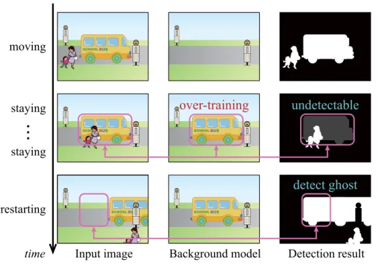
restarting

time moving

䞉䞉䞉

staying

staying undetectable

detect ghost

Detection result Input image Background model

over-training

Figure 2.4: Problems related to the appearance and disappearance of stationary objects

2.4 Detection of stationary objects

Many background models have been proposed to detect foreground objects robustly against

background changes. To model the variations in the visual appearance of the background, most

conventional approaches have used only one background model. Hereafter, the author calls this

kind of background model a single-layered background model. Then, conventional approaches

have assumed that all foreground objects keep moving and such objects can be detected using a

single-layered background model. Based on this assumption, to adapt to background changes,

conventional methods update their single-layered background model using the input image ev-

ery frame. However, this kind of maintenance of single-layered background models causes

some problems in complex situations, where not only moving foreground objects but also sta-

tionary foreground objects are observed. In a bus stop, for example, where pedestrians pass in

front of a stopped bus as shown in Figure 2.4. In such situations, the conventional single-layered

background models commonly face the following problems.

(28)

2.4 Detection of stationary objects

The appearance of stationary objects: When foreground objects stay in the same position for a long time, the single-layered background models falsely detect such objects as

“background” because they mistakenly learn the objects as “background.” In other words, the conventional background models cannot detect such foreground objects, i.e., station- ary objects, as shown in the second row of Figure 2.4.

The disappearance of stationary objects: When foreground objects move away after stay- ing in the same position for a long time, some background regions, which are occluded by the stationary object, are uncovered. Then, the conventional background models falsely detect such uncovered regions as “foreground” as shown in the third row of Figure 2.4, and these false-positive regions are called ghosts.

To address the first problem, Yang et al. [56] proposed an approach using two background models to conserve the original and the current background separately. Their approach allows to detect stopped (abandoned) objects and slow moving objects. To alleviate the second problem, Yao et al. [57] developed an updating scheme of multi-modal distributions, i.e., background model, so that the chances of forgetting old distributions corresponding to the occluded back- ground can be reduced. However, when illumination conditions change while the background regions are hidden by stationary foreground objects, their method cannot adapt to such regions.

To alleviate this drawback, Shimada et al. [58] developed an updating scheme in which original background regions hidden by foreground objects were also updated by using substitute pixels.

In practice, to update a background model of a pixel hidden by foreground object, they searched an alternative background pixel whose background model was the most similar to the hidden pixel. However, these methods [56–58] still have a problem that they cannot identify overlaps between moving foreground objects and stationary foreground objects as shown in Figure 2.5.

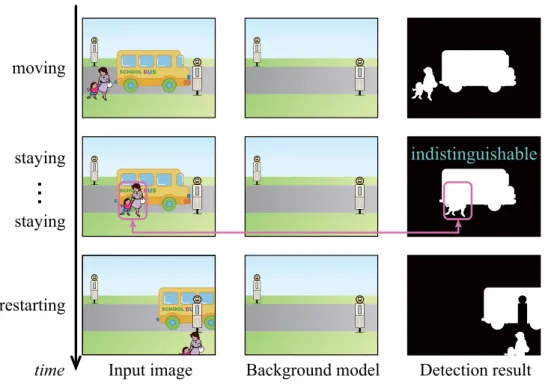
To address the problem shown in Figure 2.5, Fujiyoshi and Kanade [59] proposed a layered

detection using multiple labels. In particular, by analyzing the stabilities of pixel values, they

determined whether the agglomeration of groups of pixels belonged to a moving foreground

region or a stopped foreground region. Then, when a moving object passes in front of a stopped

(29)

Chapter 2. Related works

restarting

time moving

䞉䞉䞉

staying

staying indistinguishable

Detection result Input image Background model

Figure 2.5: Problems related to overlaps between moving foreground objects and stationary foreground objects

object, their method can discriminate overlaps between the objects. However, their method dose not adapt to background changes, because their framework cannot employ any background models. Therefore, especially in cases of outdoor surveillance, their method sometimes falsely detect the background regions affected by background changes, and then such background re- gions are mistakenly identified as abandoned or stopped objects. Additionally, their method takes much more time to adapt to the disappearance of the stationary objects than the meth- ods [57, 58], because it uses the stability analysis instead of a background model for each pixel.

Moreover, their method has difficulty recognizing pixels belonging to the same stationary ob-

ject as the same group. In [59], they basically analyze the state of each pixel independently, and

therefore, some objects are divided into several subregions.

(30)

Chapter 3 Background model based on a statistical local difference pattern

As introduced in Chapter 2, local feature-based background models [15–19, 23–29] and statistical background models [11–14, 36–53] have been proposed, but they cannot adapt to dynamic changes and illumination changes, respectively. To alleviate these problems, several hybrid background models [20–22, 54, 55] have also proposed by using multiple different back- ground models. However, hybrid methods cannot support a high recall ratio and high precision ratio at the same time, because they employed a kind of tandem system to combine the detection results of their multiple different background models.

In this chapter, the author proposes a new background model suitable for outdoor surveil- lance

¹

, by integrating the concepts of a local feature-based approach and a statistical approach into a single framework. This new framework for background modeling is the main contribu- tion of this work, and it is completely different from conventional hybrid methods. In practice, the proposed method uses illumination invariant local features, and describes their distribution by Gaussian mixture models (GMMs). The local feature has the ability to tolerate the effects of illumination changes, and the GMM can learn the multimodality of dynamic changes. There-

1

The target scenes are mainly “long shot” scenes in the outdoors, and the proposed method is not intended for

“close-up shot” scenes such that a foreground object is very large.

(31)

Chapter 3. Background model based on a statistical local difference pattern

P(x) x P(x)

x

P(x) x P(x)

x

P(x) x

Difference values

100 50 200

Gaussian Mixture Model Gaussian Mixture Model

P(x)

x

r

-20 0 50

120 50 150 Target

Target pixel pixel Neighboring Neighboring pixel pixel

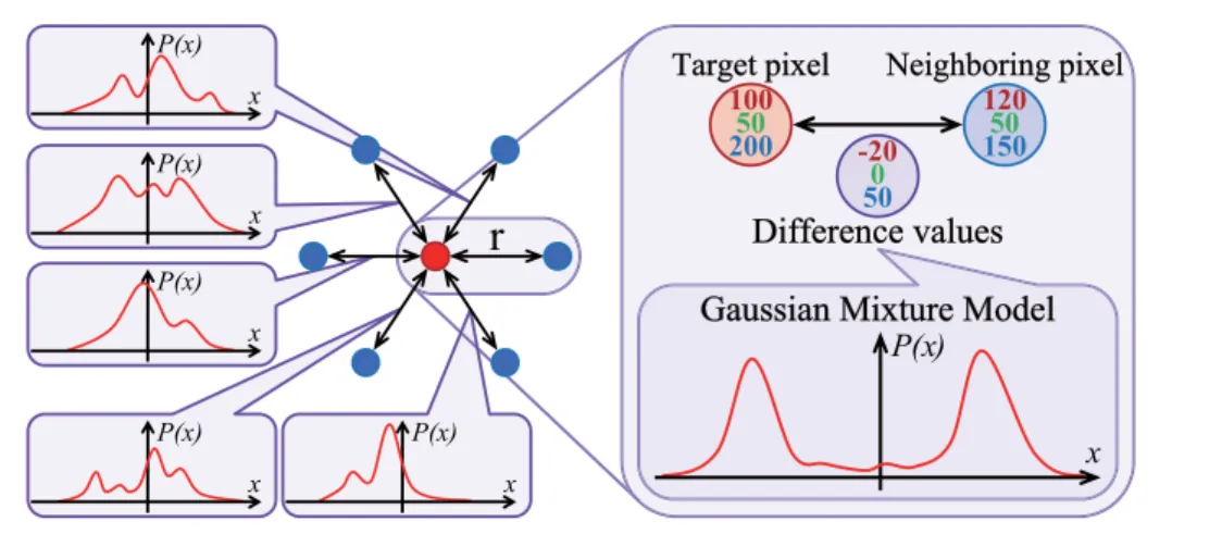
Figure 3.1: Proposed background model based on Statistical Local Difference Pattern: Local Difference (LD) is a local feature, and is defined by the difference between a target pixel and a neighboring pixel. LD is modeled using a Gaussian mixture model (GMM) to represent its distribution, making it a statistical local feature called the Statistical Local Difference (SLD).

The proposed model defines the Statistical Local Difference Pattern (SLDP) using several SLDs for the background model (this figure shows an example with six SLDs).

fore, the proposed method can detect the foreground objects robustly against both illumination and dynamic changes. This robustness against background changes is also a contribution of this work, and it can be expected that the method can support a high recall ratio and high precision ratio at the same time.

3.1 Statistical local difference pattern

In the proposed model, a GMM is applied to an illumination-invariant local feature called the

Local Difference (LD) to get a statistical local feature called the Statistical Local Difference

(SLD). Then, Statistical Local Difference Pattern (SLDP) is defined for the background model

by using several SLDs as shown in Figure 3.1. First, in Section 3.1.1, the concept and advan-

tages of SLDP are explained. Next, the construction of LD is discussed in Section 3.1.2, and

the representation of SLD using GMMs is shown in Section 3.1.3. Finally, the construction and

(32)

3.1 Statistical local difference pattern

Current frame Previous frame

- =

- ¹⁵⁷ ₂₁₄ ¹⁶⁷ =

80 120 51 -77

-163 -47

Target NeighboringDifference

221 243 240

- =

141 197 83

Target Neighboring

- 80 -160 - 43

Difference

(Difference)

X P ⁽ X )

GMM

Target Target pixel

pixel pixel pixel Neighboring Neighboring

(a) Adaptation to illumination changes

Current frame Previous frame

80 160 43 141 197 83 221

243 240 - =

221 243 240

- =

141 197 83 - 80

-160 - 43

(Difference)

X P ⁽ X )

GMM

Target NeighboringDifference Target NeighboringDifference

Target Target pixel

pixel pixel pixel Neighboring Neighboring

(b) Adaptation to dynamic changes

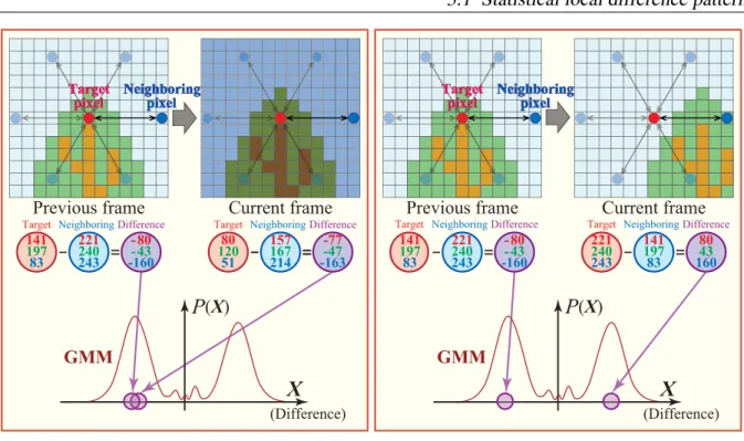
Figure 3.2: Adaptivities of the proposed model to background fluctuation: (a) shows the case of illumination changing suddenly (e.g. when sunlight is blocked by clouds). SLDP can adapt to illumination changes. This is because LD has the ability to tolerate the effects of illumination changes which affect the target pixel value in proportion with others. (b) shows the case of texture changing periodically (e.g. the effect of movement of tree or grass). GMMs can adapt to these kinds of dynamic changes, since they can learn the variety of background hypotheses.

detection rules for SLDP are explained in Section 3.1.4.

3.1.1 Concept of statistical local difference pattern

Conventional statistical approaches [11–14,36–53] can handle multimodality of dynamic changes but not illumination changes. Conversely, local feature-based approaches [17–19, 24, 25] can deal with illumination changes but not dynamic changes.

To solve these problems, the author proposes a new background model by applying a statis-

tical framework to a local feature-based approach as shown in Figure 3.1. Figure 3.2 shows the

(33)

Chapter 3. Background model based on a statistical local difference pattern

advantages of using SLDP. In most cases where illumination changes, there are small changes in the difference between a target pixel and its neighboring pixel, since the values of pixels in a localized region increase or decrease proportionally. Due to the invariance of the difference value with respect to illumination changes, SLDP has the ability to tolerate the effects of illu- mination changes as shown in Figure 3.2(a), since it uses the difference value as a local feature.

Furthermore, the proposed method can also cope with dynamic changes, since SLDP can learn the variety of the changes as shown in Figure 3.2(b). This is because a GMM, which can han- dle the multimodality of the background, is applied to LD which is an important component of SLDP. Thus, the proposed background model can integrate the concepts of both statistical and local feature-based approaches into a single framework.

3.1.2 Construction of local difference

The author defines an illumination-invariant logical feature called Local Difference (LD). Using the spatial characteristics, in which illumination changes affect not only a target pixel but also its neighboring pixels, the LD X

_j

is defined as

X

j

= f ( p

c

) − f ( p

j

) , (3.1)

where p

_c

and p

_j

are position vectors of a target pixel and its neighboring pixel in an observed image, respectively, and f ( p ) represents the pixel value of the pixel p in d -dimensional space.

Owing to the spatial characteristic, the value of LD can be stable under the illumination changes as shown in Figure 3.2(a).

3.1.3 Construction of statistical local difference

A GMM is applied to LD to represent probability density functions (PDF) for LD. This gives a statistical local feature called Statistical Local Difference (SLD). Then, the SLD P ( X

^t_j

) (PDF for LD) at time t is defined by:

P ( X

^t_j

) =

M m=1

w

_j,m^t

η ( X

^t_j

|μ

^t_j,m

, Σ

^t_j,m

) , (3.2)

(34)

3.1 Statistical local difference pattern

where w

^t_j,m

, μ

^t_j,m

and Σ

^t_j,m

are the weight, the mean and the covariance matrix of the m -th Gaussian in the mixture at time t respectively, and η is the Gaussian probability density

η ( X

^t_j

|μ

^t_j

, Σ

^t_j

) = 1

(2 π )

^d²

|Σ|

¹²

exp

− 1

2 ( X

^t_j

− μ

^t_j

)

^T

Σ

⁻¹

( X

^t_j

− μ

^t_j

)

. (3.3)

The background model can be constructed by updating the GMM (that is, the SLD). The updat- ing method for the GMM is based on the statistical approach proposed by Shimada et al. [12].

This method allows automatic changes of M , i.e., the number of Gaussian distributions, in re- sponse to background changes. That is, M increases when the background has many hypotheses because of dynamic changes, for example. On the other hand, when pixel values are constant for a while, some Gaussian distributions are eliminated or integrated, and M consequently de- creases.

3.1.4 Object detection based on a statistical local difference pattern

In the proposed method, each pixel has a pattern of SLD in the background model. In this thesis, this pattern of SLD is called Statistical Local Difference Pattern (SLDP), and SLDP S

^t

at time t is defined as follows:

S

^t

= {P ( X

^t₁

) , . . . , P ( X

^t_j

) , . . . , P ( X

^t_N

) }, (3.4) where N represents the number of SLDs (Figure 3.1 shows an example in which N = 6). The N SLDs P ( X

^t_j

) ( j = 1 , . . . , N ) are defined using a target pixel p

_c

= ( x

c

, y

c

)

^T

and N neighboring pixels p

_j

= ( x

j

, y

j

)

^T

. When a directional vector a

j

( j = 1 , . . . , N ), which describes the direction from the target pixel to each neighboring pixel, is defined as

a

_j

=

cos j − 1

N 2 π, sin j − 1 N 2 π

_T

, (3.5)

then the neighboring pixel p

_j

is given by:

p

_j

= p

_c

+ ra

j

. (3.6)

In Eq.(3.6), r is a radial distance, and all of the neighboring pixels lie on a circle of radius r

centered at a target pixel p

_c

. We can also refer to N as the number of neighboring pixels.

(35)

Chapter 3. Background model based on a statistical local difference pattern

Foreground detection using SLDP uses a voting method to judge whether a target pixel p

_c

belongs to the background or the foreground. When the pattern of N LDs is given as D

^t

= {X

^t₁

, . . . , X

^t_j

, . . . , X

^t_N

} , foreground detection based on SLDP is decided according to:

Φ( p

_c

) =

⎧ ⎨

⎩

background if φ ( D

^t

|S

^t

) ≥ T

B

, foreground otherwise ,

(3.7)

where T

B

is a threshold for determining whether a target pixel p

_c

belongs to the background or the foreground. In Eq.(3.7), φ ( D

^t

|S

^t

) is a function which returns a value between 0 and N , and is defined by

φ ( D

^t

|S

^t

) =

N

j=1

ψ ( X

^t_j

) , (3.8)

where ψ ( X

^t_j

) is a function which returns 0 or 1, depending on whether or not the LD X

^t_j

matches the SLD P ( X

^t_j

) at time t . The LD is said to match the SLD if it falls within 2.5 standard deviations of the mean. For further details, please refer to Appendix A.

3.2 Experimental results

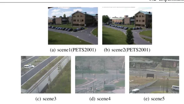
In this section, two types of experiments were conducted. In the first experiment, the overall foreground detection performance using SLDP was compared with three different background modeling approaches. The datasets for the five outdoor scenes illustrated in Figure 3.3 were used for this evaluation. As we can see from Figure 3.3, they are long shot scenes, and are the targets for the SLDP. Scene1 and scene2 are taken from PETS (PETS2001)

²

, and scene3, scene4 and scene5 are from LIMU datasets which are available from the website

³

. The PETS datasets involve not only pedestrian movement though the streets, but also illumination changes (sunlight blocked by clouds) and dynamic changes, such as fleeting clouds and the swaying motion of tree leaves, in the background. The LIMU datasets include several different sizes of

2

Benchmark data of the International Workshop on Performance Evaluation of Tracking and Surveillance.

Available from ftp://pets.rdg.ac.uk/PETS2001/

3

Several kinds of test image are available from http://limu.ait.kyushu-u.ac.jp/dataset/

(36)

3.2 Experimental results

(a) scene1(PETS2001) (b) scene2(PETS2001)

(c) scene3 (d) scene4 (e) scene5

Figure 3.3: The datasets for evaluation

moving objects such as pedestrians, cars, buses, etc. After that, the validity of SLDP for object detection is evaluated using Wallflower [54] dataset

⁴

.

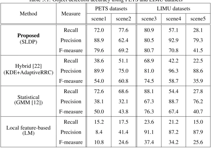
3.2.1 Comparison with conventional background modeling approaches

In this subsection, the overall performance of foreground detection using SLDP is compared with three different methods, the GMM method [12], the Local Magnitude (LM) method and the hybrid method [22]. The GMM method removes the local feature-based framework from SLDP, and is consistent with a statistical approach using Gaussian mixture model [12]. The LM method removes the statistical framework from SLDP, and models local magnitude relations between a target pixel and its neighboring pixels. The hybrid method [22] combines a statistical model based on KDE and a local feature-based model using an AdaptiveRRC which is an adaptive version of RRC [19]. Here, the GMM and LM methods were used to evaluate the effectiveness of the statistical and local feature-based approaches, respectively. The hybrid method [22] was used to indicate that the SLDP is better than hybrid approaches which used the ad hoc solutions by a logical combination.

4

Wallflower dataset contains images and their ground truth data for various background subtraction issues.

(37)

Chapter 3. Background model based on a statistical local difference pattern

Table 3.1: Object detection accuracy using PETS and LIMU datasets

Method Measure PETS datasets LIMU datasets

scene1 scene2 scene3 scene4 scene5 Proposed

(SLDP)

Recall 72.0 77.6 80.9 57.1 28.1

Precision 88.9 62.4 80.5 92.9 79.3

F-measure 79.6 69.2 80.7 70.8 41.5

Hybrid [22]

(KDE+AdaptiveRRC)

Recall 38.6 51.1 68.9 42.2 22.5

Precision 89.9 75.0 81.0 96.3 88.6

F-measure 54.0 60.8 74.5 58.7 35.9

Statistical (GMM [12])

Recall 72.6 68.6 88.1 54.4 27.8

Precision 38.1 32.1 67.3 88.7 76.2

F-measure 50.0 43.8 76.3 67.4 40.7

Local feature-based (LM)

Recall 15.2 17.5 23.6 21.2 15.0

Precision 8.4 41.4 91.1 87.2 87.9

F-measure 10.8 24.6 37.4 34.2 25.6

In these experiments, the radial distance is r = 10, the number of neighboring pixels is N = 6 and the detection threshold is T

B

= 5. Although the details of GMM are not explained in Section 3.1.3, the author also indicates the parameter settings in GMM for reproducibility:

the learning rate is α = 0 . 05, the initial weight is W = 0 . 05 and the threshold of choosing the background model T = 0 . 7. For the details of GMM, please refer to Appendix A. Table 3.1 shows performance evaluation results for foreground detection using manually-produced ground truth datasets

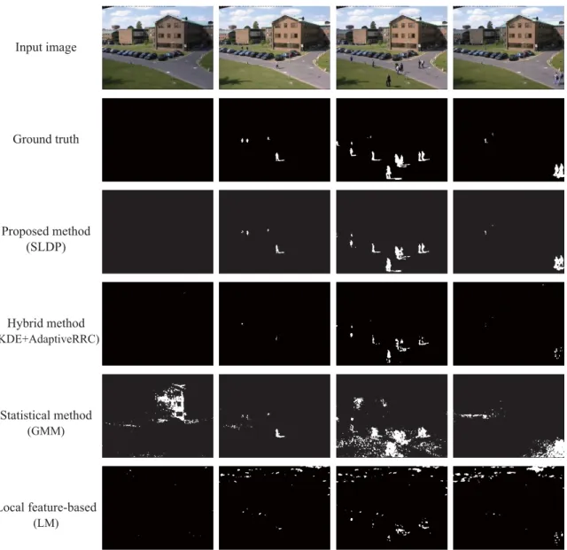
⁵

based on Recall, Precision and F-measure. To demonstrate the experi- mental results, some results of foreground detection for scene1 are also shown in Figure 3.4.

This PETS datasets includes illumination changes and dynamic changes. Therefore, Table 3.1

5

A ground truth image denotes the foreground regions which should be detected by background subtraction.

The ground truth datasets for several benchmark datasets, including those used in this thesis, are published on

http://limu.ait.kyushu-u.ac.jp/dataset/

(38)

3.2 Experimental results

Input image

Ground truth

Proposed method

Hybrid method

Statistical method

Local feature-based (SLDP)

(KDE+AdaptiveRRC)

(GMM)

(LM)

Figure 3.4: Examples of foreground detection results using a PETS dataset (scene1)

(39)

Chapter 3. Background model based on a statistical local difference pattern

shows that precision values of the GMM and LM methods are low for PETS datasets. In the case of GMM, it cannot adapt to illumination change and detects a number of noises as shown in the fifth row of Figure 3.4. In the case of LM, it cannot adapt to dynamic changes, and the last row of Figure 3.4 shows that LM detects a lot of false-positive pixels (note especially the area of sky). On the other hand, Table 3.1 shows that the SLDP and the hybrid method both achieve high precision ratios for the PETS datasets, since they can adapt to both illumination and dy- namic changes. Therefore, little noise is detected in the third and fourth rows of Figure 3.4, which further shows that these methods can adapt to both types of background change.

In the cases of LIMU datasets (scene3, 4 and 5), neither illumination changes nor dynamic changes are severe. Therefore all of the methods achieve a high precision ratio for these datasets in Table 3.1. In terms of the recall ratio, however, there are differences between the methods in Table 3.1. In the case of the LM method, it is robust against illumination changes, but it has difficulty detecting entire foreground objects because the operator is too simple. Therefore, Table 3.1 shows that the LM method has the lowest recall ratio for all scenes. Table 3.1 also shows that the recall ratio for the hybrid method is lower than for the SLDP and for the GMM.

This is because the hybrid method combines the results of multiple different models using a

logical AND operation, and false-negative pixels in either of the two models reduce the true-

positive rate. This is also confirmed in the fourth row of Figure 3.4, in which there are a lot of

false-negative pixels in the object regions. Conversely, in the cases of the SLDP and the GMM,

their models can be constructed using a single framework, and therefore they maintain a high

recall ratio. As a result, Table 3.1 shows that the SLDP and the GMM both achieve a high

recall ratio over whole scenes. For these reasons, the author concludes that the SLDP can use

the aspects of both local feature-based and statistical approaches more effectively compared to

conventional hybrid approaches.

(40)

3.2 Experimental results

Table 3.2: Performance evaluation using Wallflower dataset

Scene Wallflower [54] Proposed (SLDP)

False-negative False-positive False-negative False-positive

Moved object 0 0 0 0

Time of Day 961 25 791 44

Light Switch 947 375 2369 280

Waving Trees 877 1999 600 788

Camouflage 229 2706 8887 387

Bootstrapping 2025 365 1439 132

Foreground aperture 320 649 2690 553

Total Errors 11478 18960

3.2.2 Validation using Wallflower dataset

In this subsection, to investigate what kind of scenes the SLDP can handle apart from its target scenes, Wallflower dataset [54] is used. This dataset contains not only long shot scenes but also close-up shot scenes which observe a large foreground, and includes the background changes which are not observed in the outdoor. Regarding the parameters, the same ones used in Section 3.2.1 are employed. The visual and numerical results are shown in Figure 3.5 and Table 3.2 respectively, in which the results of Wallflower are cited from its literature [54]. In Table 3.2, the row of total errors indicates the summation of false-negative and false-positive pixels in each scene.

With respect to total errors, the performance of the SLDP is lower than Wallflower. This is because the SLDP detects many false-negative pixels in three close-up shot scenes: “Light Switch,” “Camouflage” and “Foreground Aperture,” as shown in Figure 3.5 and Table 3.2.

These close-up shot scenes are not the targets for the SLDP, and it is difficult to robustly detect

the foreground objects. One reason for this is that the SLDP does not model the background

color but rather the difference between a target pixel and its neighboring pixels. In most cases

(41)

Chapter 3. Background model based on a statistical local difference pattern

(a) Input image Light Switch

(d) Proposed (SLDP) (c) Wallflower

(b) Ground truth Bootstrapping

Waving Trees Time of Day

Camouflage Moved Object

Foreground Aperture

Figure 3.5: Foreground detection results using Wallflower dataset

(42)

3.3 Summary

of close-up shot scenes, the background has a uniform texture, and then the change in the SLDP is hardly-detectable when an object with a uniform texture appears. Therefore, the SLDP mistakenly regards the foreground object as the background in the close-up shot scenes, and that is a limitation of the SLDP. Another reason is that the SLDP has no post-processing for complementing the object regions with a homogeneity such as color similarity. In the case of Wallflower, as the post-processing phase, it complements the object regions with color sim- ilarity and can achieve a reduction of false-negative pixels. If some post-processing such as Graph-Cut, morphological operations, etc., are used, it can be expected the proposed method can also reduce the number of false-negative pixels.

On the other hand, in scenes other than those listed above, the SLDP can outperform Wallflower as we can see from Figure 3.5 and Table 3.2. This is because these scenes except for “Waving Trees” are long shot scenes, and “Waving Trees” has a relatively complicated tex- ture in its background. Then the SLDP can distinguish the object regions from the background without confusing the object with the background as discussed above. These scenes also involve illumination and dynamic changes in the background. The SLDP can adapt to both changes, and therefore the proposed method detects few false-positive pixels. From the results of Sec- tion 3.2.1 and this section, it can be confirmed that the proposed method can detect foreground objects accurately in the long shot scenes and the scenes which have a relatively complicated texture in their background.

3.3 Summary

In this chapter, the author has proposed a new background model based on the Statistical Local

Difference Pattern (SLDP). The main contribution of this work is proposing a method that in-

tegrates the concepts of a local feature-based approach and a statistical approach into a single

framework. In the proposed framework, the SLDP uses illumination-invariant local features

which have the ability to tolerate the effects of illumination changes, and describes their distri-

bution by GMMs which can learn the multimodality of dynamic changes. Then, this modeling

(43)

Chapter 3. Background model based on a statistical local difference pattern

framework allows the SLDP to have both properties of local feature-based and statistical ap-

proaches, and SLDP can adapt to both illumination changes and dynamic changes in the back-

ground. As shown in the experimental results, we have confirmed that the SLDP can detect the

foreground objects robustly against illumination changes and dynamic changes, especially in

long shot scenes.

複雑環境下における物体検出のための背景モデリン グ

九州大学学術情報リポジトリ

Kyushu University Institutional Repository