流体力学におけるクローン波動関数の応用2例 (オイラー方程式の数理 : 力学と変分原理250年)

(1)

Two

applications

of

Coulomb

wave

functions

in

hydrodynamics

(

流体力学におけるクーロン波動関数の応用

2 例

)

Takahiro

Nishiyama

(

西山高弘

)

Department ofApplied Science, Yamaguchi University, Ube 755-8611, Japan e-mail: [email protected]

1 Introduction

The regular Coulomb wave function $F_{L}(\eta, \rho)$ for $L\in N\cup\{0\},$ $\eta\in \mathbb{R}$ and $\rho>0$ is

defined by

$F_{L}(\eta, \rho)=C_{L}(\eta)\rho^{L+1}e_{1}^{-i\rho}F_{1}(L+1-i\eta;2L+2;2i\rho)$ $=(2i)^{-(L+1)}C_{L}(\eta)M_{i\eta,L+1/2}(2i\rho)$,

where $1F_{1}$ and $M$ denote Kummer’s and Whittaker‘s regular confluent hypergeometric

functions, respectively, and

$C_{L}( \eta)=\frac{2^{L}|\Gamma(L+1+i\eta)|}{e^{\pi\eta,2}(2L+1)!}=\{\begin{array}{ll}\frac{2^{L}}{(2L+1)!}\sqrt{\frac{2\pi\prod_{k=0}^{L}(k^{2}+\eta^{2})}{\eta(e^{2\pi\eta}-1)}} for \eta\neq 0,\frac{2^{L}L!}{(2L+1)!} for \eta=0,\end{array}$

[1, Chapter 14], [3, Appendix I.A.14]. The value of $F_{L}(\eta, \rho)$ is real because of the

Kummer transformation

$e^{-i\rho_{1}}F_{1}(L+1-i\eta;2L+2;2i\rho)=e^{i\rho_{1}}F_{1}(L+1+i\eta;2L+2;-2i\rho)$

[1, Eq. 13.1.27]. If $\eta$ is aconstant, then $w(\rho)=F_{L}(\eta, \rho)$ is a solution to $\frac{d^{2}w}{d\rho^{2}}+[1-\frac{2\eta}{\rho}-\frac{L(L+1)}{\rho^{2}}]w=0$.

As another solution to this equation that is independent of $F_{L}(\eta, \rho)$, the irregular

Coulomb

wave

function $G_{L}(\eta, \rho)$ is defined by

$G_{L}( \eta, \rho)=\frac{(\pm 2i)^{2L+1}\rho^{L+1}e^{\mp i\rho}}{C_{L}(\eta)(2L+1)!}\Gamma(L+1\mp i\eta)U(L+1\mp i\eta, 2L+2, \pm 2i\rho)\pm iF_{L}(\eta, \rho)$

(2)

so

that $G_{L}( \eta, \rho)\frac{d}{d\rho}F_{L}(\eta, \rho)-F_{L}(\eta,\rho)\frac{d}{dp}G_{L}(\eta,\rho)=1$

.

Here $U$ and $W$denote Kummer’s

and Whittaker $s$ irregular confluent hypergeometric functions, respectively. There

are

various formulas for $F_{L}(\eta, \rho)$ and $G_{L}(\eta, \rho)$ in [1]. In particular, the

case

$L=\eta=0$ is

easy: $F_{0}(0,\rho)=\sin\rho$ and $G_{0}(0,\rho)=\cos\rho$

.

Coulomb

wave

functions

are

mainly used in quantum physics, especially in

scat-tering theories (see [8], and rcferences therein, e.g. [7, Chapter III]). In the field of

hydrodynamics, howcver, therc

are

only a few papers using them. In this article, two

applications of Coulomb

wavc

functions in hydrodynamics

are

introduced. One is to

an

orthogonal series associated with steady Euler flows (\S 2), and the other is to the

stability problem for pipe Poiseuille flow (\S 3).

2 An

orthogonal

series

associated with steady

Euler

flows

When

an

Euler flow istwo-dimensional and in

a

steady state, then it is described by a stream function $\psi(x, y)$

as

$\frac{\partial^{2}\psi}{\partial x^{2}}+\frac{\partial^{2}\psi}{\partial y^{2}}=-g(\psi)$

with

an

arbitrary differentiable function $g$ [$2$, Section 7.4]. It is clear that each basis

function of the two-dimensional Fourier series satisfies this equation with $g$ linear.

Therefore, the two-dimensional Fourier series can be regarded

as

a superposition of

steady planar Euler flows.

Similarly, asteadyaxisymmetric Euler flow isdescribedbya Stokesstream function

$\phi(r, x)$ in the cylindrical coordinate system $(r, \theta, x)$

as

$r \frac{\partial}{\partial r}(\frac{1}{r}\frac{\partial\phi}{\partial r})+\frac{\partial^{2}\phi}{\partial x^{2}}=-r^{2}h(\phi)$

ifthe $\theta$-component of velocity is equal to

zero

[2, Section 7.5]. Here $h$ is

an

arbitrary

differentiable function. If$h$is linear, then

$r \frac{\partial}{\partial r}(\frac{1}{r}\frac{\partial\phi}{\partial r})+\frac{\partial^{2}\phi}{\partial x^{2}}=-\lambda r^{2}\phi$ (1)

with a constant $\lambda$. What is an orthogonal series whose basis functions mean steady

axisymmetric Euler flows?

Set $\phi=\Phi(r)e^{2:}\mathfrak{n}\pi x/b(n\in \mathbb{Z}, b>0)$ in (1). Then $\Phi(r)$ should satisfy

$r \frac{d}{dr}(\frac{1}{r}\frac{d\Phi}{dr})-4(\frac{n\pi}{b})^{2}\Phi+\lambda r^{2}\Phi=0$

.

(2)

As mentioned byHerrnegger [5] and Maschke [6], it has a solution

(3)

when $\Phi(0)=0$ is imposed. The author [9], [10] pointed out that there exists a set $\{\lambda_{m,n}\}(m\in N)$ for eachfixed $n\in \mathbb{Z}$ and a constant$a>0$ such that _{$R_{\eta}^{n}(\sqrt{\lambda_{m,n}};a)=0$}

and

$( \frac{2n\pi}{ab})^{2}<\lambda_{1,n}<\lambda_{2,n}<\lambda_{3,n}<\cdots$ .

Furthermore, using the Hilbert-Schmidttheory, he deduced that $\{m(\sqrt{\lambda_{mn}};r)\}(m\in$

N$)$for eachfixed_$n$isacomplete orthogonal systemon$(0, a)$ with the weightfunction

$r$.

In otherwords, every function $f(r)$ that satisfies $\int_{0}^{a}[f(r)]^{2}rdr<\infty$

can

berepresented

in the form

$f(7^{\cdot}) \sim\sum_{m=1}^{\infty}R_{0}^{n}(\sqrt{\lambda_{mn}};r)\frac{\int_{0}^{a}R_{0}^{n}(\sqrt{\lambda_{mn}};t)f(t)tdt}{\int_{0}^{a}[R_{0}^{n}(\sqrt{\lambda_{mn}};t)]^{2}tdt}$ (3)

in the square integrable space with the weight $r$.

In consequence, thc set $\{\phi_{m,n}(r, x)\}:=\{R_{t^{n}}(\sqrt{\lambda_{mn}};r)e^{2in\pi x/b}\}(m\in N, n\in \mathbb{Z})$ is a

complete orthogonal system with the weight $r$

on

$(0, a)\cross(-b/2, b/2)$ such that each

basis expresses a steady axisymmetric Euler flow. It should be noted that the author [10] derivcd

an

integral transform whose kernel is a Stokes streamfunction ofa steady axisymmetric Euler flow by letting $aarrow\infty$ and $barrow\infty$.

Notingthat

$\int_{0}^{a}[R_{t}^{n}(\sqrt{\lambda_{mn}};r)]^{2}rdr=\frac{A_{m,n}B_{m,n}}{2a\sqrt{\lambda_{mn}}}$

is valid for

$A_{m,n}= \frac{d}{dr}m(\sqrt{\lambda_{mn}};r)_{r=a}$, $B_{m,n}= \frac{\partial}{\partial u}R_{\eta}^{n}(u;a)_{u=\sqrt{\lambda_{mn}}}$

[10, Eq. (4.1)], wecanprove the followingtheorem, whichis a more specificresult than (3):

Theorem 1 ([11]).

_If

$\int_{0}^{a}|f(t)|tdt<\infty$ and the total vareation

of

$f$ is bounded on

$[\alpha_{1}, \alpha_{2}]\subset(0,a)$, then

$\frac{f(r-0)+f(r+0)}{2}=2a\sum_{m=1}^{\infty}\frac{\sqrt{\lambda_{mn}}}{A_{m,n}B_{m,n}}R_{0}^{n}(\sqrt{\lambda_{mn}};r)\int_{0}^{a}R_{0}^{n}(\sqrt{\lambda_{mn}};t)f(t)tdt$

for

all

_fixed

$r\in(\alpha_{1}, \alpha_{2})$ and$n\in \mathbb{Z}$.

The proofis doneby extending $F_{L}(\eta, \rho)$ and _{$G_{L}(\eta, \rho)(L=0$}or 1$)$ tocomplex

$\eta$ and $\rho$. It is similar to the proof ofWatson $f20$, Sections 18.$21-18.24J$ on the Fourier-Bessel

series, the best-known orthogonal series with the weight function $r$

.

Because of the

gammafunction, howcver, Coulomb wave functions with complex arguments

are

more delicate to treat than Bessel functions.

(4)

3Stability problem for pipe Poiseuille flow

Thc stability problcm for pipe Poiseuilleflow has a long history. The analytical study

of its dcpendcnce

on

the Reynolds number $R$

was

started by Sexl [17]. After that,

many researchers investigated behavior of small disturbances to the pipe flow ffom various theoreticalvicwpoints and deduced the linear stability at every $R$ (see [4], and

references therein). It was Pekeris [13] who first applied a confluent hypergeometric function (i.e.

a

Coulomb

wave

function with complex arguments) to the stability anal-ysis of pipe Poiseuilleflow. Sexl

&

Spielberg [18] followed. In this section, byusing the result ofasymptotic analysisof Skovgaard [19],

we

consider thedistributionofcomplex phase velocities for small axisymmetric torsional disturbances to pipe Poiseuille flow.

Let $\Omega(r)$ be afunction such that $\Omega(r)e^{i\alpha(x-d)}/r$ is anormal mode for axisymmetric

torsional disturbancesto the pipe flow whichhas the velocity $1-r^{2}(0<r<1)$ in the x-direction in the cylindrical coordinate system $(r, \theta,x)$. Here the wave-number $\alpha>0$

and the complex phase velocity $c\in \mathbb{C}$

are

constants. Pekeris [13] derived the linearized

equation of the same type

as

(2):

$7^{\cdot}$$\frac{d}{dr}(\frac{1}{r}\frac{d\Omega}{dr})-\alpha^{2}\Omega-i\alpha R(1-r^{2}-c)\Omega=0$

with the boundary conditions $\Omega(1)=0$ and $| \lim_{rarrow+0}\Omega(r)/r|<\infty$. Setting

$\kappa=\frac{1}{4}[\frac{\sqrt{\alpha R}(1-c)}{e^{i\pi/4}}-\frac{\alpha^{2}e^{i\pi/4}}{\sqrt{\alpha R}}]$ ,

we solve it

as

$\Omega(r)\propto F_{0}(\kappa,e^{i\pi/4}r^{2})\propto F_{0}(-i\kappa,$ $- \frac{1}{2}\sqrt{\alpha R}e^{1\pi/4}r^{2})$

$\propto\mu(\alpha, R, c;r):=M_{\kappa,1/2}(\sqrt{\alpha R}e^{-i\pi/4}r^{2})$

with

$\mu(\alpha, R, c;1)=0$

.

(4)

This (4) determines the value of $c$ for given $\alpha$ and $R$. If $R|1-c|arrow\infty$ with $\alpha$ fixed,

then $\kappa$ is asymptotically equal to $k$ defined by

$k= \frac{\sqrt{\alpha R}(1-c)}{4e^{i\pi/4}}=\frac{\sqrt{\alpha R}}{4|z|}e^{-i(\arg z+\pi/4)}$,

where $z=1/(1-c)$. Therefore, in the limit

$\sqrt{R}|1-c|arrow\infty$ and $R|1-c|arrow\infty$ with $\alpha fixed$, (5)

we have $|k|arrow\infty$ and $\mu(\alpha, R, c;1)\sim M_{k,1/2}(4kz)$, to which the result of asymptotic

(5)

${\rm Im} z$

Figure 1: The sets $D_{1},$ $D_{2}^{\pm}$ and $\ell$ of

$z$, and the corresponding sets of$c=1-1/z$.

Let us make ready for stating asymptotic forms of$\mu(\alpha, R, c;1)$. As proved in [13],

every $c(=c_{r}+ic_{\dot{\tau}})$ of (4) satisfies $0<c_{r}<1$ and _{$c_{i}<0$}. Consequently, $z$ should

belong to one of the three sets

$D_{1}= \{s:-\pi/2<\arg s<-\pi/4, |s-\frac{1}{2}|>\frac{1}{2}, |s|<\infty\}$ , $D_{2}= \{s:-\pi/4<\arg s<0, |s-\frac{1}{2}|>\frac{1}{2}, |s|<\infty\}$ ,

$l= \{s:\arg s=-\pi/4, |s-\frac{1}{2}|>\frac{1}{2}, |s|<\infty\}$.

We define the function $\xi$by

$\xi(z)=\{\begin{array}{ll}\frac{1}{2}z^{1/2}(z-1)^{1/2}-\frac{1}{2}\ln[z^{1/2}+(z-1)^{1/2}]-i\pi/4 for z\in D_{1},\frac{1}{2}z^{1/2}(z-1)^{1/2}-\frac{1}{2}\ln[z^{1/2}+(z-1)^{1/2}] for z\in D_{2}\cup\ell.\end{array}$

Here, and from

now

on, multivalued functions should be understood to take their

principal values. Using this $\xi$, we divide $D_{2}$ into the two sets

$D_{2}^{+}=\{s\in D_{2}:{\rm Im}\xi(s)\geq 0\}$, $D_{2}^{-}=\{s\in D_{2} : {\rm Im}\xi(s)<0\}$.

Figure 1 shows the locations of $D_{1},$ $D_{2}^{\pm}$ and $\ell$ on the z-plane and the corresponding

sets on the c-plane. It also shows the point $z=\rho_{0}e^{-i\pi/4}\in l$ with $\rho_{0}\approx 2.1844$, at

which $\arg\xi(z)=-\pi/2$ holds, and _the _{corresponding point}

(6)

Wc

now

express asymptotic forms of$\mu(\alpha, R,c;1)$ in the limit (5)

as

follows:

$\mu(\alpha, R, c;1)\sim 2(-\xi)^{1/2}(\frac{z}{z-1})^{4}I_{1}(4k\xi)1$ for $z\in D_{1}$, (7)

$\mu(\alpha, R,c;1)\sim\frac{2^{2/3}3^{1/6}\xi^{1/6}e^{*\pi(k-2/3)}}{k^{1/3}}(\frac{z}{z-1})^{1/4}Ai((6k)^{2/3}\xi^{2/3}e^{-2\cdot\pi/3})$

for $z\in D_{2}^{-}$, (8) $\mu(\alpha, R,c;1)\sim\frac{2^{5/3}3^{1/6}\xi^{1/6}e^{1\pi/6}\sin\pi k}{k^{1/3}}(\frac{z}{z-1})^{1/4}Ai((6k)^{2/3}\xi^{2/3}e^{2i\pi/3})$

for $z\in\ell$ with $|z|>\rho_{0}$. (9)

Here$I_{1}$ denotes the first-kind modffied Besselfunctionof the first order, andAidenotes

the Airy function. The case $z\in D_{2}^{+}$ or $z\in\ell$ with $|z|\leq\rho_{0}$ is omitted because the

asymptotic form has no zero. For details of the derivation of (7)$-(9)$,

see

[19], and also

[12].

The

zeros

of the right hand sides of (7)$-(9)$ approximately determine $c$ of (4) in

the limit (5). Since all zeros of $I_{1}$ and Ai

are

located

on

the imaginary axis and thc

negative real axis, respectively, the equality $\arg(k\xi)=-\pi/2$ is necessarily satisfied by

all $z$ that make the right hand side of (7) or (8) vanish. It leads to

$\arg\{z^{1/2}(z-1)^{1/2}-\ln[z^{1/2}+(z-1)^{1/2}]-\frac{i\pi}{2}\}-\arg z+\frac{\pi}{4}=0$ for $z\in D_{1}$, (10)

$\arg\{z^{1/2}(z-1)^{1/2}-\ln[z^{1/2}+(z-1)^{1/2}]\}-\arg z+\frac{\pi}{4}=0$ for $z\in D_{2}^{-}$. (11)

Moreover, as another neccssary condition for $\mu(\alpha, R,c;1)$ to vanish approximately,

we

add

$|z|>\rho_{0}$ for $z\in\ell$, (12)

under which

_the.factor

$\sin\pi k$ in (9) has

zeros

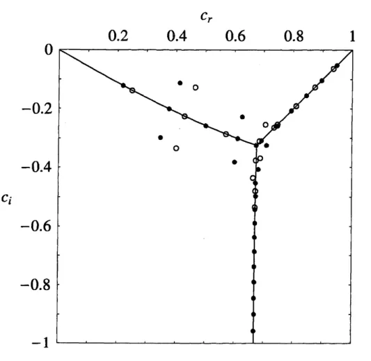
(while Ai in (9) has no zero). By

numerically solving (10) and (11) with respect to $c=1-1/z$ and adding the straight

linesegment given by (12), weobtainthe Y-shaped contour shown in figure2, onwhich

zerosof$\mu(\alpha, R, c;1)$

are

approximatelylocated. Thethree branches ofthis contourmeet

at a point $c=c_{0}$, alrcady appeared in (6) and figure 1. Figure 2 shows the locations

of $c$ computed by Schmid

&

Henningson [15, Table 1, $n=0$], $[16, p.506, n=0]$,

too. Most of them

are

on or near the Y-shaped contour. Although

some

are off the leftward branch ofthc contour, they

are

not of torsional disturbances but of meridional disturbances (see [14, Figure 2]). It should be noted that the Y-shaped structure in figure 2 is independent of$\alpha$ and $R$. Of course, the location of each individual $c$of (4)

depends on $\alpha$ and $R$,

as

investigated in detail in [12]. In particular, about $c_{\tau}\approx 2/3$ on

the downwardbranch of the contour, the followingtheorem

can

beanalyticallyproved:

Theorem 2 ([12]).

_If

$\alpha$ and$R$ are

fixed

at arbitrarypositive numbers, then there exist

(7)

0.2

$c_{r}$

0.4

0.6

0.8

1

Figure 2: The Y-shaped contourobtained from (10)$-(12)$, with $c$ computed by Schmid

&

Henningson [15], [16] for $R=3000$ $(\bullet$ $)$ and $R=2000(0)$ when $\alpha=1$.

Acknowledgment

The author thanks Professor Yuji Hattori for his information about [5] and [6].

References

[1] M. Abramowitz, I. A. Stegun, Handbook

_of

Mathematical Functions, with Formu-las, Gmphs, and Mathematical Tables, U. S. Government Printing Office, 1964. [2] G. K. Batchelor, AnIntroduction to FluidDynamics, Cambridge University Press,

1967.

[3] H. Buchholz, The

_Confluent

Hypergeometric Function, Springer, 1969.

[4] P. G. Drazin, W. H. Reid, Hydrodynamic Stability, Cambridge University Press,

(8)

[5] F. Herrnegger, On the equilibrium and stability of the belt pinCh, Proceedings

_of

the

_Fifth

European

_Conference

on

Controlled Rasion and Plasma Physics,

Greno-ble, France, August 21-25, 1972, vol. 1, p. 26.

[6] E. K. Maschke, Exact solutions of the MHD equilibrium equation for a toroidal

plasma, Plasma Phys. 15 (1973) 535-541.

[7] N. F. Mott, H. S. W. Massey, The Theory

_of

Atomic Collisions, Clarendon, 1933. [8] National BureauofStandards, Tables

_of

Coulomb Wave Functions, U. S.

Govern-ment Printing Office, 1952.

[9] T. Nishiyama, Construction of axisymmetric steady states of

an

inviscid

incom-pressible fluidby spatiallydiscretizedequations for pseudo-advectedvorticity, Int. J. Math. Math. Sci. 2005 (2005) 3319-3346.

[10] T. Nishiyama, Anintegraltransformwhosekernel is astreamfunction ofasteady

Euler flow with axisymmetry, Z. Angew. Math. Phys. 58 (2007) 68-80.

[11] T. Nishiyama, Application of Coulomb

wave

functions to

an

orthogonal series

associated with steady axisymmetric Euler flows, J. Approx. Theory 151 (2008)

42-59.

[12] T. Nishiyama, Distribution of complex phase velocities for small disturbances to

pipe Poiseuille flow, J. Fluid Mech. 620 (2009) 299-312.

[13] C. L. Pekeris, Stability of the laminar flow through a straight pipc of circular

cross-section to infinitesimal disturbances which

are

symmetrical about the axis

of the pipe, Proc. Nat. Acad. Sci. USA 34 (1948) 285-295.

[14] W. H. Reid, B. S. Ng, On the spectral problem for Poiseuille flow in a circular pipe, Fluid$Dyn$. Res. 33 (2003) 5-16.

[15] P. J. Schmid, D. S. Henningson, Optimal energy density growth in Hagen-Poiseuille flow, J. Fluid Mech. 277 (1994) 197-225.

[16] P. J. Schmid,D. S. Henningson, Stability and 71nansitionin ShearFlows, Springer, 2001.

[17] T. Sexl, ZurStabilit\"atsfrage dcr Poiseuilleschen undCouetteschenStr\"omung, Ann.

Phys. 83 (1927) _835-848.

[18] T. Sexl, K.Spielberg, Zum $Stabilittsproblem$derPoiseuille-Str\"omung, ActaPhys.

Austriaca 12 (1958) 9-28.

[19] H. Skovgaard,

_Unifom

Asymptotic Expansions

_{of Confluent}

Hypergeometric Functions and Whittaker Functions, Jul. Gjellerups, 1966.

$[20|$ G. N. Watson, A 7heatise on the Theory

of

Bessel Functions, 2nd edition,