Stochastic Control of
Fishery
ResourcesUsing Dynamical
Models forLocal Behaviour andGlobalPopulation
(局所的行動と大域的個体群の動態モデルを用いた水産資源の確率制御)
Hidekazu
Yoshiokal,,
YutaYaegashi,
KoichiUnami,
andMasayukiFujihara2
1
Facultyof Life andEnvironmentalScience,ShimaneUniversity,Japan
2
Graduate SchoolofAgriculture, Kyoto University, Japan
*\mathrm{E}‐mail:[email protected]‐u.ac.jp
1. Introduction
Ecologically‐conscious fisheryresources management is currentlyamajor issue all over the world.
Designingandcarryingoutanappropriatemanagementplanofmigratoryfishspeciesinariver,which
aremajorinlandfisheryresources,requirescomprehendinghydrologicalandhydrauliccharacteristics
of their habitatsand migrationprocesses. An example of such fish species is Plecoglossus altivelis
(Ayu)livinginJapan,which isakey aquatic speciesin thecountryfromeconomical, ecological, and culturalviewpoints [1‐3]. Hugetransverse hydraulic structures installedacross river cross‐sections,
whichare oftenequipped withfishways to improve passageefficiency offishes, serve as physical
barriers forupstreamfishmigration [4].Aweirnotequippedwithanyfishwaysorthose withpoorly
designed fishways possibly fragmentsariverintohydraulicallydisconnectedreaches [5]. Operatinga
largedam for humanactivitieswouldsignificantlyalter its downstreamriver environmentand leadto
regimeshifts ofhydraulic [6]andecologicalconditions in rivers[7],both of whichcriticallyaffect life
histories of migratory fishes [8‐9]. Establishment of an effective management strategy for the
migratoryfishspeciesshouldconsidercomplex ecologicaland environmentalsystemsthataffect their migrationandhabitation.Ecosystem dynamicsisinherently subjecttostochastic enviromnentalnoises resulting from complex internal and external interactions [10‐11]. From this standpoint, stochastic
process modelscanpotentiallyserveas effective mathematicaltools toanalyze, predict, and control
both localswimmingbehaviourandglobal populationdynamicsofmigratoryfishspecies.
Fishmigrationinwaterbodies have oftenbeenanalyzedwithindividual‐Uased models thattrack
movementsofindividual fishes inwaterbodies [12, 13].\mathrm{M}\mathrm{o}\mathrm{s}\mathrm{t}ofsuch models havetoapriorispecify
theswimming velocityas afunctionofhydraulic variables,which wouldactuallybedynamicallyand adaptivelycontrolledbythe individual fish itselfduringits migrationprocess. Yoshioka et al. [14]
proposedamathematicalmodel ofupstreamfishmigrationofindividual fishes in1‐Drivers basedon
astochastic differentialequation (SDE)combined withadynamic programming principle [15]. Their
mathematicalmodelassumesthattheoptimal swimmingvelocityof individualfishes is the minimizer
of a value function based onboth biological and ecological considerations. Finding the optimal
swimming velocity reduces to solving a Hamilton‐JacoUi‐Uellman equation (HJBE), which is a
nonlinear and nonconservativepartialdifferentialequation (PDE) [15]. Mathematical and numerical
analysesonsolutionstotheHJBEgoverningupstreamfishmigrationfromtheviewpointofviscosity
solution[16]have beenperformed [17, 18].The authors alsoanalyzedstochasticpopulationdynamics
of released migratory fishes in a river system subject to predation pressure from waterfowls and fishingpressurefrom humanusingadifferentHJBEderived fromaneconomic andecologicalvalue
population dynamicsmodels,haveindividuallybeendevelopedandanalyzed; however, weconsider
thatsomelinkscanbe foundbetween thetwomodels,which isamain motivation ofthispaper.
The mainobjectiveofthispaper istopresenttheabove‐mentionedmigration dynamicsmodeland
population dynamicsmodel,andtoconsider linksbetweenthem Therestof thispaper isorganizedas
follows.Section2brieflyintroducesastochasticcontroltheorytoderiveanHJBE fromanSDE based on a dynamic programming principle. Section 3 presents the migration dynamics model and the population dynamicsmodel discussed in this paper. Section4presents demonstrative computational examplesofthesemodelsfocusingontheirapplìcationstofisheryresourcesmanagementin HiiRiver,
San‐inarea,Japan. Section5 discusseslinks betweenthetwomodels. Section 6concludes thispaper
andpresentsfutureperspectivesofourresearch.
2. Stochasticcontrol theorv
2.1 Stochasticdifferential equation
Toformulatetheupstreamfishmigration, alltheprocesses and randomvariablesaredefinedonthe
usual filteredcomplete probabilityspacewitharight‐continuous filtration \mathcal{F}_{t} [15]. Consider an n
‐dimensional real‐valued continuous stochastic process
\mathrm{X}_{t}=[X_{\mathrm{i},t}]
(1\leq i\leq n) in the boundeddomain $\Omega$\in \mathbb{R}^{n} with theboundary \partial $\Omega$ where
t(\geq 0)
is thetime. Theboundary (isr2 containstheabsorbingboundary \partial$\Omega$_{\mathrm{A}} andthereflectingboundary \partial$\Omega$_{\mathrm{R}}, which donotintersectwith eachother.
The stochasticprocess \mathrm{X}_{t} isassumedtobeacontrolledMarkov process. Itis assumed thatthe initial
condition
\mathrm{X}_{0}^{\cdot}=\mathrm{x}=[x_{i}]
is deterministically specifiedatthe time t=0. Thegoverning equationof\mathrm{X}_{\mathrm{t}} inthe domain $\Omega$ is theItôs SDE
\mathrm{d}\mathrm{X}_{t}=\mathrm{a}(t,\mathrm{X}_{t},u_{l})\mathrm{d}t+b(t,\mathrm{X}_{t},u_{l})\mathrm{d}\mathrm{B}_{l}
(1)where
\mathrm{B}_{\mathrm{t}}=[B_{i,t}]
is the n‐dimensionalstandardBrownian motion [15], u_{t} is thecontrol variablethatbelongsto anadmissiblesetof control
\ovalbox{\tt\small REJECT}=L^{\infty}([0,+\infty
)
;U)
with the range U,\mathrm{a}=[a_{i}]
is then‐dimensionaldriftcoefficient vector,
b=[b_{i,j}]
is the nx n‐dimensionaldiffusivitymatrix that isassumedtobenon‐negativedefinite. Theinfinitesimalgenerator A^{u} associated withtheSDE(I) is
expressedforgeneric sufficientlyregularfunction
\emptyset= $\phi$(s,\mathrm{x})
asA^{u} $\phi$=\displaystyle \sum_{i=1}^{n}a_{i}\frac{\partial $\phi$}{\partial x_{i}}+\sum_{jj,=1}^{n}D_{i,j}\frac{\partial^{2}\emptyset}{\partial x_{i}\partial$\kappa$_{j}}
(2)with
D_{i,j}=\displaystyle \frac{1}{2}\sum_{k=1}^{n}b_{i.k}b_{k,j}
.The variable u_{\mathrm{t}} is assumedtobeaMarkovcontrol.2.2 Value function
In the stochastic control theory, the objective function to be maximized through choosing an
appropriatecontrol variable u_{t} isexpressedas[15]
v(s,\displaystyle \mathrm{x},u)=\int_{s}^{\overline{T}}f(t,X_{\mathrm{t}},u_{t})\mathrm{d}t+g(\overline{T},X_{\overline{T}}) , \overline{T}=\dot{\mathrm{m}}\mathrm{f}(T, $\tau$)
(3) withthe firsthittingtime $\tau$ definedas$\tau$=\mathrm{m}\mathrm{f}\{t|t>s,\mathrm{X}_{s}=x,\mathrm{X}_{l}\in\partial$\Omega$_{\mathrm{A}}\}
(4)where f and g representtheprofit (orthecost)pertimeunit and thatgainedatthe terminal time
T,respectively.Thegoalof thestochasticcontrolproblemistofindanoptimalcontrol u=u^{*}\in \mathscr{K}
that maximizes anexpectationoftheobjectivefunction. Themaximizedobjectivefunction umderthe
expectationis referredtoasthe valuefunction,which isexpressedas
$\Phi$(s,\displaystyle \mathrm{x})=\sup_{u\in ff}\mathrm{E}[v(s,\mathrm{x},u)]=\mathrm{E}[v\left(s,\mathrm{x},u & *\right)]
(5)with
u=\displaystyle \mathrm{a}r\mathrm{g}\max_{u\mathrm{e}A}\mathrm{E}[v(s,\mathrm{x},u)]
(6)where \mathrm{E} representstheexpectation.
2.3 Hamilton‐Jacobi‐Bellmanequation
Application ofthe dynamic programming principle [15] to the value function in (5) leads to the goveming equationofthe value function $\Phi$,which,is theHJBEexpressedas
\displaystyle \frac{\partial $\Phi$}{\partial s}+\sup_{u\in U}\{A^{u} $\Phi$+f(s,\mathrm{x},u)\}=\frac{\partial $\Phi$}{\partial s}+A^{u} $\Phi$+f\left(s,\mathrm{x},u & *\right)=0
\mathrm{i}\mathrm{n} $\Omega$ (7) subjecttotheboundaryconditions\displaystyle \frac{\partial $\Phi$}{\partial \mathrm{n}}(s,\mathrm{x})=0
for 0<s<T and \mathrm{x}\in\partial$\Omega$_{\mathrm{R}} (8)and
$\Phi$(s,\mathrm{x})=g(s,\mathrm{x})
for 0<s<T and \mathrm{x}\in\partial$\Omega$_{\mathrm{A}}, (9)and theterminalcondition
$\Phi$(T,\mathrm{x})=g(s,\mathrm{x})
\mathrm{i}\mathrm{n} $\Omega$ (10)where
\displaystyle \frac{\partial}{\partial \mathrm{n}}=\sum_{i=1}^{n}n_{i}D_{i,j}\frac{\partial}{\partial x_{j}}
and\mathrm{n}=[n_{i}]
is the outward normal vector on the boundary \partial $\Omega$. Forstationary problemswherethe coefficientsand value functionsaretime‐independent, (7) reducesto
A^{u} $\Phi$+f(s,\mathrm{x},u^{*})=0
\mathrm{i}\mathrm{n} $\Omega$ (11)subjecttotheboundaryconditions (8) and (9).
3. Mathematical model 3.1 Mitration dvnamics model
TheSDE that governshorizontally2‐D swimmmngbehaviourof individual fishes in ariver reach is
considered in thissection.Inthedomain $\Omega$\in \mathbb{R}^{2} of shallowwaterflows, the2‐Dstochasticprocess \mathrm{X}_{t} describesapositionofanindividual fishateach time t.Theswimming velocity
\mathrm{u}_{t}=(u_{1,\mathrm{t}},u_{2,t})
\mathrm{d}\mathrm{X}_{l}=(\mathrm{V}(t,X_{t})-\mathrm{u}_{t})\mathrm{d}t+b(t,X_{t},u_{l})\mathrm{d}\mathrm{B}_{\mathrm{t}}
(12)where V is the 2‐D flow velocity vector and the 2‐D square matrix b modulates stochastic
swimmingbehaviourofthe fish. TheSDE(12) isaspatially2‐Dextension ofthe1‐D model[17].The
positive direction of \mathrm{u} is taken opposite to that of V to focus on upstream fish migration.
Experimentalresults suggest that the diffusivity matnix D would bea decreasingfunction of the
swimming speed
|\mathrm{u}|
[20]; however, here it is assumed not to depend on|\mathrm{u}|
for the sake ofsimplicity. Itis also assumed thatthecoefficients V and b aretime‐independent given functions,
which can be valid when considering the migration with significantly shorter timescale than
hydrological changesof river flows.
The range U of the control \mathrm{u} issetasthe2‐Dclosedball
|\mathrm{u}|\leq u^{(\mathrm{M})}
, (13)which is based on thetrivial fact that the fish has abiologicallydeterminedmaximum swimming speed u^{(\mathrm{M})}. Yoshioka et al. [17, 21] consideredanHJBE associatedwith the 1‐D model assuming
unbounded u^{(\mathrm{M})} and found thattowell‐posetheproblem requires regularizationofanonlinearterm,
which artificiallytruncates theswimming speed. Therefore, boundedness of u^{(\mathrm{M})} is areasonable
assumptionfromboth mathematicalandbiological viewpoints.
The valuefunction
$\Phi$= $\Phi$(\mathrm{x})
,which isassumedtobetime‐independent,issetas$\Phi$(\displaystyle \mathrm{x})=\sup_{\mathrm{u}\mathrm{e}\ovalbox{\tt\small REJECT}}\mathrm{E}[v(\mathrm{x},\mathrm{u})]
(14)with theobjectivefunction
v(\displaystyle \mathrm{x},\mathrm{u})=-\int_{0}^{r}f(\mathrm{u}_{\mathrm{t}})\mathrm{d}t+g(\mathrm{X}_{ $\tau$})
(15)where
f(\displaystyle \mathrm{u}_{t})=\frac{1}{m+1}|\mathrm{u}_{l}|^{m+1}
(16)with m\geq 1 represents the consumedphysiological energy per time duringthe migration, which is
assumedtobeanincreasingandconvexfunctionof theswimming speed followingthe theoreticaland
experimental results [22, 23], and
g(\mathrm{X}_{ $\tau$})
represents the profit obtained when approaching the absorbing boundary \partial$\Omega$_{\mathrm{A}} atthe firsthittingtime $\tau$.Theabsorbing boundary \partial$\Omega$_{\mathrm{A}} isdecomposedinto the upstream boundary \partial$\Omega$_{\mathrm{A}\mathrm{U}} where the flow is inward (\mathrm{V}\cdot \mathrm{n}<0) and the downstream
boundary \partial$\Omega$_{\mathrm{A}\mathrm{D}} wherethe flow is outward(\mathrm{V}\cdot \mathrm{n}>0).Thereflectingboundary \partial$\Omega$_{\mathrm{R}} in thepresent caserepresentsthewallboundarywherethe flow doesnotpenetrate(\mathrm{V}\cdot \mathrm{n}=0).It is alsoassumed that noprofitis obtainedat thedownstreamboundary \partial$\Omega$_{\mathrm{A}\mathrm{D}}(g=0).
Applicationof thedynamic programming principleto (14) leadstothe HJBE
\displaystyle \sum_{i=1}^{n}(V_{i}-\mathcal{U}_{i}^{*})\frac{\partial $\Phi$}{\partial x_{\dot{ $\eta$}}}+\sum_{:}^{n}D_{i,j}\frac{\partial^{2} $\Phi$}{\partial x_{i}\partial x_{j}}-\frac{1}{m+1}|\mathrm{u}|^{m+1}ij=1=0
\mathrm{i}\mathrm{n} $\Omega$ (17) withtheoptimal swimmingvelocity \mathrm{u}^{n} as afunctionof thegradientofthevaluefunction \nabla $\Phi$:\displaystyle \mathrm{u}^{*}=-\frac{\nabla $\Phi$}{|\nabla $\Phi$|}\mathrm{m}\mathrm{j}\mathrm{n}\{u^{(\mathrm{M})},|\nabla $\Phi$|^{\frac{1}{m}}\}
in $\Omega$. (18)The gradient \nabla $\Phi$ thus determines both the direction and magnitude of the optimal swimming
velocity \mathrm{u} .Heuristically,the fish swims with themaximumswimming speed u^{(\mathrm{M})} where
|\nabla $\Phi$|
islargerthan u^{(\mathrm{M})} andswims with thespeed
|\nabla $\Phi$|^{\frac{1}{m}}
when|\nabla $\Phi$|
is smaller thanu^{(\mathrm{M})}.
3.2 Population dvnamicsmodel
The stochastic processmodel for annual population dynamics of releasedP. altivelis in ariver is
presented following Yaegashiet al. [19]. Let
(0,T)
with the terminal time T be aperiod duringwhichthepopulation dynamics of releasedP. altivelis inariver is considered. The initialtime t=0
and theterminal time t=T aresetin thespringand theautumnwithinayear,respectively.The total
biomass of P. altivelis in this river at the time t is denoted as the 1‐D non‐negative continuous
stochasticprocess X_{\mathrm{t}}.The initial condition X_{0} atthetime t=0
,whichis thereleaseamountof the
juveniles,is assumedtobe deterministic. Thisisvalid for thecasewheremostpartof thepopulation
of P.altivelis in the riverisintroducedthroughintensivereleaseevents.The initialpopulation X_{0} is
expressedas X_{0}=NW_{0} where N is thenumberofindividuals releasedatthe time t=0 and W_{0}
is theaverageweightof thejuvenilesatthat time.ThegoverningItôs SDEof the stochasticprocess
X_{\mathrm{t}} isgivenas
\mathrm{M}_{t}=(a(t,X_{l})-l_{l}X_{t})\mathrm{d}t+b(t,X_{l})\mathrm{d}B_{\ell}
withl_{t}=R+k(u_{l})+$\chi$_{\{l\geq T_{\mathrm{c}}\}}c_{\mathrm{t}}
(19)and thegrowth‐curvebased Verhulstmodel[24, 25]
a(t,x)=r(1-K^{-1}X_{t})X_{t}
andb(t,x)= $\sigma$ X_{t}
(20)where B_{\mathrm{t}} is the 1‐D standard Brownianmotion[15], R is the naturalmortalityrate,
k(u_{t})
is thepredationpressurefromawaterfowlas afunction oftheefforttoreduce the pressure u=u_{t}, c isthe
fishing pressure fromhuman, T_{\mathrm{c}}<T is theopening time ofharvesting P altivelis,and $\chi$_{s} is the
characteristic function for genericset S. Thecapacity K
,the intrinsicgrowthrate r,and the noise
intensity $\sigma$ arepositivemodelparameters. The noise intensity a implicitlymodels influences of
the natural and artificial environmental changes in the river to the population dynamics as a
multiplicative noise.[26]. Assumingthat thepopulation dynamics is limitedbythereleased amount
ratherthanbythe enviromnentalcapacity,theparameter K isexpressedas[19]
K=M_{0}=mNW_{0} (21)
withapositiveconstant m.Thisassumptioncanbevalid forariver where thepopulationofreleased
P.altivelis dominates thenaturalcounterpartsandtheydonot saturatein thehabitat.
The variables u and c aretakenasthecontrolsvariables in the model.The admissiblesetof
the controls u and c are
\mathrm{a}=L^{\infty}([0,+\infty
)
;U)
andC=L^{\infty}([0,+\infty
)
;C)
, respectively. The rangeU and C ofthecontrols u and c arespecifiedas
U=\{u|0\leq u\leq 1\}
andC=\{c|0\leq c\leq c_{\mathrm{M}}\}
, (22)v=v(s,x,u,c)
is assumed to represent the profit of the local fisherycooperatives. The objectivefunctionisproposedas
v=\displaystyle \int_{s}^{T}\{-f(u_{t})+$\chi$_{\{t\geq T_{\mathrm{c}}\}} $\theta$ c_{t}X_{\mathrm{t}}\}\mathrm{d}t- $\eta$ X_{0}
(23)where
f(\geq 0)
withf(0)=0
isanincreasing function, $\theta$ is thepriceofmaturedP. altivelisperweightand $\eta$ isthecostoflarval P. altivelisperweight,both ofwhichareassumedtobeconstant.
Thefirst and secondintegrandsofEq.(23) arethe costofoperatingcountermeasures toexterminate
thepredatorandthe total benefitofharvestingP. altivelis,respectively. Theterm - $\eta$ X_{0} represents
thecost tobuylarval P. altivelistobereleasedatthe time t=0.Thetwofunctions
k(u)
andf(u)
onthe control variable u aresimply specifiedas
k(u)=k_{0}(1- $\alpha$ u)
andf(u)=0Xl
, (24)respectivelywhere k_{0} isthepredationpressure from thewaterfowl withoutanycoumtermeasures, a
with 0<a\leq 1 modulates efficiencyto decrease thepredationpressure withthe control u, and $\omega$
modulatesthecost todecrease thepredationpressure.
Thevaluefunction ispresentedas
$\Phi$(s,x)=\displaystyle \sup_{u\in Z/,c\in \mathcal{C}}\mathrm{E}[v(s,x,u,c)]
(25)whosegoverningHJBE is
\displaystyle \frac{\partial $\Phi$}{\partial s}+\sup_{u\in$\theta$^{!},c\in \mathcal{C}}\{A^{u,c} $\Phi$-f(u)+$\chi$_{\{s\geq T_{\mathrm{c}}\}} $\theta$ cx\}=\frac{\partial $\Phi$}{\partial s}+A^{u.\mathcal{C}} $\Phi$-f(u^{*})+$\chi$_{\{s\geq T,\}}$\theta$_{\mathcal{C}^{*}}x=0
in $\Omega$ (26)wheretheoptimalcontrols u^{*} and c^{*} via thevalue function $\Phi$ as
u^{*}=1(k_{0} $\alpha$ r- $\omega$\geq 0)
, u^{*}=0(Otherwise)
andc^{*}=c_{\mathrm{M}}( $\theta$ x- $\gamma$\geq 0)
, c^{*}=0(Otherwise)
, (27)respectivelywhere
$\gamma$=x\displaystyle \frac{\partial $\Phi$}{\partial x}
. Bothof theoptimalcontrolsarethus thebang‐bangtype.Thedomainof thepopulationof P. altivelis x is setas
$\Omega$=(0,L)
withL(>0)
determined later. Substitutingu=u^{*} and c=c into (26) fully specifiestheHJBEin thedomain $\Omega$. The terminalcondition for
the HJBE is setas $\Phi$_{s=T}=0 and theboundaryconditions as V_{\mathrm{x}=0}=0 and
\displaystyle \frac{\partial $\Phi$}{\partial x}|_{x=L}=0
.SolvingtheHJBEyieldstheoptimalcontrols u^{*} and c^{*} over
(0,T)\mathrm{x}(0,L)
.4. Applications
4.1 Studvarea
Demònstrative application examplesof themigrationdynamicsmodel andpopulationdynamicsmodel
focusingonP. altivelisin HiiRiver,San‐in area,Japanarepresented. Populationofthe fish in the river
isthoughttohave beenconsiderablydecreasingduetodegradationofriver environmentbydam and
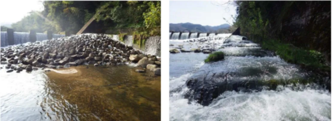
weir constructions and excessive predationpressure from waterfowls: Phalacrocorax carbo (Great Cormorant) [27, 28] (Photo. 1). The total lengthof the mainstream and the catchmentarea of Hii
Photo 1: P. altivelis(left panel)and P. carbo(right panel).
(The photo\mathrm{o}\mathrm{f}P.carbo is taken from\mathrm{h}\mathrm{t}\mathrm{t}\mathrm{p}://\mathrm{w}\mathrm{w}\mathrm{w}.yunphoto.\mathrm{n}\mathrm{e}\mathrm{t}).
described and analyzed in detail in Sato et al. [30, 31], and not explained in this paper. Two
downstream brackish lakes named LakeShinjiand Lake Nakaumi fromupstreamareconnectedtothe river. Beingdifferent from thecasesof the rivers thatdirectlyflow into thesea,hatched larvae of P.
altivelis are thought to descend to Lake Shinji; however, it is not well‐known where they survive
duringwinterseason.
4.2 Migration dvnamicsmodel
The HJBE for the migration dynamics model is applied to numerical computation of spatial distribution of the optimal swimming velocity of individual P. altivelis in the downstreamarea of
Yoshii Weir installedatamidstream reach of HiiRiver,which isaweirtocontrolchannel erosion with the width of 80 (m)and theheightof 3 (m) (Photo 2).Afieldsurvey carriedoutbythe authorsduring June,2015 found that the mainstream of Hii River hasanumber of weirs and Yoshii Weir isrelatively
larger one among them. Photo 3 shows fishways currentlythat are installed to Yoshii Weir. The
previousYoshiifishwayconsistedsolelyof thepool‐type fishway.Downstreampoolsof thisfishway suffered fromseveredepositions of fine soilparticles. This mightbe duetoits geometryofshaping flow recirculation thattrapstheparticles. Suchdepositionswereconsideredtobea causeofdegrading
fluidtransportcapacityof thefishway,whichmighthave further leadtodegradationof its attraction
ability and passage efficiency for migratory fish species. The downstream part of the pool‐type
fishwaywasrenovated in 2013 in ordertoreduce the sedimentdeposition.Around thesametime, the nature‐like fishway was installed at the same side of the weir so that migratory fishes can more
efficientlyfind the waytopassage the weir. Currently,Hii River FisheriesCooperatives,who manage
fisheryresources in middle andupstreamreaches of Hii River, areconcerned with attraction ability
and passage efficiency of the renovated Yoshi Weir. Assessing attraction ability and passage
efficiencyof the weir is thereforeahighly importantissue.
A2‐Dtime‐independentshallowwaterflow field in the domain isnumerically computedwith the 2‐Dshallowwaterequations usingthe verified finite element/volume scheme[32]. Thecomputational domainwasextracted from GoogleEarth(Google Inc., MountainView, Calif.) has been discretized into57,443 triangularelements and 113,609nodesusingthe free software named VORO(availableat
http://wwwyss‐aya.com/voro.html). The HJBE isnumerically solved with a 2‐D counterpartof the Petrov‐Galerkin finite element scheme[33] that has alreadybeen verified withsimplerHJBEs. The
maximum swimming speed u^{(\mathrm{M})} is set as 2 (\mathrm{m}/\mathrm{s}), which is approximately same with the burst
swimming speedobserved atlaboratorial experimental results [34]. Theparameter m for the cost
function isset tobe 3consideringthe identification result basedonlaboratorialexperiments [17]. The
downstream‐end of the domain is consideredasthe downstreamboundary \partial$\Omega$_{\mathrm{A}\mathrm{D}}.Theentranceof the
pool‐type fishwayand thetop of the nature‐like fishwaywhere the individual fishes canpassageare
consideredastheupstreamboundary \partial$\Omega$_{\mathrm{A}\mathrm{U}}.Theremainingparts of theboundary \partial $\Omega$ is considered as the reflecting boundary \partial$\Omega$_{\mathrm{R}} . The value function $\Phi$ is specified as $\Phi$=0 on \partial$\Omega$_{\mathrm{A}\mathrm{D}} and
$\Phi$=P_{0}
(
=const>0)
on \partial$\Omega$_{\mathrm{A}\mathrm{U}} where P_{0} is the ecological profit to be gained on \partial$\Omega$_{\mathrm{A}\mathrm{U}}. Theparameter P_{0} is set as
P_{0}=20,000(\mathrm{m}^{4}/\mathrm{s}^{3})
. Preliminary computational investigations impliedthattheoptimal swimming velocity \mathrm{u}^{*} doesnotsignificantly dependonthe
P_{0}>10,000(\mathrm{m}^{4}/\mathrm{s}^{3})
;namely,\mathrm{u}^{*} is almostindependentof P_{0} when it issufficiently large.Thistendencyof \mathrm{u}^{*} is consistent with the theoreticalanalysisresults for the 1‐D model [18].Asteadystatenumerical solution iscomputed withaPicard iteration method forsolvingnonlinearequations.
Figures 1(\mathrm{a}) through 1(\mathrm{d}) show the computational results with the migration dynamics model.
Figures 1(\mathrm{a}) and 1(\mathrm{b})presentthecomputedflow field basedonthe shallowwaterequations, which
qualitatively agree with field observation results. Figures 1(\mathrm{c}) shows the computedvalue fUnction whose maximum value is normalizedto 1 and the optimal swimming velocityvectors. Figure 1(\mathrm{d})
shows the expectation of the first hitting time $\tau$ of the individual fishes from each point in the
domain $\Omega$ toeither of thetwoopen boundaries(theentranceof thepool‐type fishwayandthetopof the nature‐likefishway). Figure 1(\mathrm{d})indicates that thecomputationalresults show that the firsthitting time hasasharpinteriorlayer alongthe downstream of Yoshii Weir. As indicated inFigure 1(\mathrm{c}),this
is consideredtobe duetothat individual fishes areattractedtothecurrentsfrom Yoshi Weirserving
as areflecting boundary. Thecomputationalresultsimplythat thecurrentfrom thepool‐type fishway
is too weakto attractthemigratingfishes. The individual fishes atdownstream of thelayermay be
able to find the entrance of the pool‐type fishway with non‐zero, but very small probability. In
addition,the flowspeedin the nature‐likefishwayistoohighforfishestoascend:exceedingalmost 3
(\mathrm{n}\sqrt{}\mathrm{s}),which islargerthan
u^{(\mathrm{M})}=2(\mathrm{r}\mathrm{r}\sqrt{}\mathrm{s})
. Thepresented computationalresultssuggestapossibilitythat thecurrentfishwaysarenoteffectively workingaspassages for P. altivelis.
thepool‐type fishway (right panel).Both of the
photographsaretaken from downstream.
Figure 1: Computed water depth (upper left panel), water surface elevation and horizontal flow
velocityvectors(upper right panel),value function and theoptimal swimming velocityvectors (lower
4.3 PoIJulation dvnamicsmodel
Thepopulation dynamicsmodel isappliedtonumericalcomputationofoptimalstrategyforharvesting and extermination of P. carbo in ordertosustain released P. altivelispopulationin Hii River. Table 1 summarizes theparametervalues determined basedoninformation from officers in Hii RiverFishery
Cooperatives. On the other parameters, the natural mortality rate R is estimated as 4.6\times 10^{-3}
(1/\mathrm{d}\mathrm{a}\mathrm{y})[35]. The value of a is estimatedas 0.50 [19]. The maximumfishingpressure c_{\mathrm{M}} is set as0.01 (1/\mathrm{d}\mathrm{a}\mathrm{y}) following Yaegashietal. [19]and it haspreliminarybeen checked that thisparameter doesnot significantlyaffectqualityof the value function and the controls than the otherparameters.
Assuming that the SDE (19) with k=c_{\mathrm{M}}=0 admits a non‐trivial and non‐singular probability
densityforlarge T[36],the range ofthe noiseintensity $\sigma$ issetas
0.04\leq $\sigma$\leq 0.32(1/\mathrm{d}\mathrm{a}\mathrm{y}^{1/2})
.Thevalue of theparameter k_{0} is estimated from anexactsolutionto adeterministic counterpart of the
SDE(19) with c_{\mathrm{M}}=0 andgiven X_{0} for eachcomputation ] 19[. Basedontheweights of matured
and released P. altivelis[37, 38] theparameters r, $\sigma$, and X_{0} aresetas
6.8\times 10^{-2}(1/\mathrm{d}\mathrm{a}\mathrm{y})
, 0.18(1/\mathrm{d}\mathrm{a}\mathrm{y}^{1/2})
, and 2,250 (kg), respectively. The domain of the population of P. altivelis x is set as$\Omega$=(0,6.0\times 10^{4})
(kg) andis uniformlydiscretized into a mesh with 300 elements and 301 nodes.The time increment fortemporal integrationis 0.01 (day). TheHJBE(26) isnumericallysolved with the verified Petrov‐Galerkin finite element scheme[33]. Increasing computationalresolution in space and time doesnotsignificantlyaffect thecomputationalresultspresentedbelow.
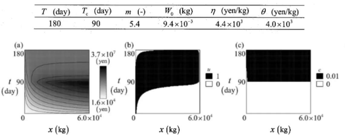
The optimal management strategy is numerically computed for a set of parameters as a
demonstrative example. Figures 2(a) through 2(c) plot the computed value function $\Phi$ and the
optimal controls u^{*} and c^{*}, respectively. Figure 2(a) shows that the value function $\Phi$ does not
have spurious oscillations, indicating that the numerical scheme canreasonably handle the HJBE.
Figure 2(b)shows that theoptimalstrategyfor the extermination of P. carbo istointensivelyreduce thepredationpressuremainly after theopeningtime T_{\mathrm{c}} exceptthe terminal time T,and before the
openingtime T_{c} for thecaseof small biomass of P. altivelis. Figure 2(c)indicates that the optimal
harvestingstrategyistoharvest P. altivelis after theopeningtime T_{\mathrm{c}} exceptfor smallpopulation x.
Table 1:Specifiedvalues ofthe modelparametersin thepopulation dynamicsmodel.
\overline{\frac{T(\mathrm{d}\mathrm{a}\mathrm{y})T_{\mathrm{c}}(\mathrm{d}\mathrm{a}\mathrm{y})m(-)W_{0}(\mathrm{k}\mathrm{g}) $\eta$(\mathrm{y}\mathrm{e}\mathrm{n}/\mathrm{k}\mathrm{g}) $\theta$(\mathrm{y}\mathrm{e}\mathrm{n}/\mathrm{k}\mathrm{g})}{180905.49.4\times 10^{-3}4.4\times 10^{3}4.0\times 10^{3}}}
\bullet u1
\bullet c0.01
口 0 口0
10^{4} 0 6.0\times 10^{4}
x
(kg)
x(kg)
x(kg)
Figure 2: Computational results of(a)value function $\Phi$, (b) optimalefforttoreduce thepredation
5. Linksbetweenthe two models
Themigration dynamicsmodeland thepopulationdynamicsmodeldeal withthedynamicsoffishery
resources in rivers based on different spatial and temporal scales. The migration dynamics model
tracks local swimmingbehaviourofmigratoryindividual fishes in riverflows,while the population
dynamicsmodelassessestemporalevolution of thepopulationof thefishesinriversashabitats.There
shouldbesome links between thetwomodels sincetheydescribethesamedynamics fromdifferent
viewpoints. The authors consider that it is possible to see the population dynamics model as a
coarse‐scaledmigrationdynamicsmodel.Spatially‐distributedstatistics,suchasascending probability
andfirsthittingtime ofindividualfishes forphysicalbarriers,computedwiththemigration dynamics
model wouldbeusedfor identifyingthe modelparameters r, K,and $\sigma$ in thepopulation dynamics
model. Inaddition,theabove‐mentionedtwostatistics aredirectlyrelatedwithmigrationrateof the
fishes between habitatspartially fragmented by physicalbarriers. Considering hydraulic regimes at
andaround thephysicalbarrierscansupportreasonably evaluatingtheirattractionabilityandpassage
efficiency.Amulti‐habitatcounterpartof thepopulation dynamics model,aspresentedin the literatureJ
[39],canthen bedevelopedwithsuch localand crucialecologicalinformation.
6. Conclusions
Astochastic controltheorywasappliedto dynamic mathematical modelling oflocalmigration and
global population dynamicsofmigratoryfishes in river environment. Themigrationdynamicsmodel assumedanenergyminimizationprincipletodetermine theoptimal swimming velocityofindividual
fishes in shallow water flow fields. The population dynamics model considers temporal biomass
changes ofreleasedfisheryresourcesin river environmentsubjecttoharvestbyhuman andpredation
from waterfowls. Linkages between the two models were discussed focusing on physical barriers
installedacrossriver cross‐sections.
Futureresearches willaddress mathematical and numericalanalyses ofthemodels, their further
practical applications, and their improvements for more realistic analysis of fishery resources
dynamics. For example, objective functions, coefficients, and parameters involved in each mathematical model shouldmoreclosetorealistic basedonavailable field survey data and testimonies
from field workers. So far, Yoshioka et al. [40] addressed identification of more. biologically
reasonablecost functionfor themigration dynamics model,whichhas beenappliedto anumber of
migratoryfishspecies.
Acknowledgements
This research is supportedbythe RiverFund inchargeof TheRiverFoundation andJSPS Research
Grant No. 15\mathrm{H}06417. Apartof thisresearchincludes research resultsfrom theshort‐stayresearcher
project in 2015 ofInstitute of Mathematics for Industry, Kyushu University, Japan. Wethankto
officers of CivilEngineering DepartmentoftheGovernment of ShimanePrefecture,Hii‐RiverFishery
Cooperatives, Yonago Waterbirds Sanctuary, and the Ministry of Environment for their valuable
commentsandprovidingdata. Wealso thanktoDr.KayokoKamedaof LakeBiwa Museum and Mr.
Kohei Yokota,Mastercourse graduatestudentof GraduateSchool ofAgriculture, Kyoto University
References
[1] MAFF (2015) Statistics ofcatch andproductionamoumts ofaquaticresources inJapanduring
2015. \underline{\mathrm{h}\mathrm{t}\mathrm{t}\mathrm{o}://\mathrm{w}\mathrm{w}\mathrm{w}.\mathrm{m}\mathrm{a}\mathrm{f}\mathrm{f}.\mathrm{g}\mathrm{o}.\mathrm{i}\mathrm{D}/\mathrm{i}/\mathrm{t}\mathrm{o}\mathrm{k}\mathrm{e}\mathrm{i}/\mathrm{s}\mathrm{o}\mathrm{h}\mathrm{A}\mathrm{o}\mathrm{u}/ $\epsilon$ \mathrm{v}\mathrm{o} $\sigma$ \mathrm{v}\mathrm{o}\mathrm{u}\mathrm{s}\mathrm{e}\mathrm{i}\mathrm{s}\mathrm{a}}\mathrm{n}_{-}13/----\cdot Last accessed on July 11,
2015.(in Japanese).
[2] Takahashi, I. andAzuma, K. (2006):TheUp‐to‐now KnowledgeBook ofAyu, Tsukiji‐shokan,
Tokyo. (in Japanese).
[3] Tanaka, Y., Iguchi,K.,Yoshimura,J.,Nakagiri,N., andTainaka, K. (2011) Historicaleffectin
theterritorialityofayufish,Journal of TheoreticalBiology, 268(1), pp.98‐104.
[4] Iwasaki, A. and Yoshimura, C. (2012): Effect of river fragmentationby crossing structures on
probabilityofoccurrenceoffreshwater fishes,Joumal ofJapan Societyof CivilEngineers, Ser. Bl,68(4),pp.\mathrm{I}_{-}685-\mathrm{I}_{-}690.
[5] Grill, G., Dallaire, C.O.,Chouinard,E.F., Sindorf, N.,andLehner,B.(2014) Developmentofnew
indicatorstoevaluateriverfragmentationand flowregulationatlargescales:a casestudyforthe
MekongRiverBasin, EcologicalIndicators, 45,pp.148‐159.
[6] Wang, Z.B., Van Maren, D.S., Ding, P.X., Yang, S.L., Van Prooijen, B.C., De Vet, P.L. M.,
Wmterwerp, J.C., De Vriend H.J., Stive, M.J.F., and He, Q. (2015) Human impacts on
morphodynamicthresholdsinestuarinesystems,ContinentalShelf Research(in press).
[7] Holt, C.R., Pfitzer, D., Scalley, C., Caldwell,B.A.,andBatzer,D. P.(2014)Macroinvertebrate community responses to anmual flow variation from riverregulation: An 11‐year study, River Research andApplications. (in press).
[8] Braaten, P.J.,Elliott, C.M.,Rhoten, J.C., Fuller, D.B.,andMcElroy,B.J. (2015) Migrationsand swimmmng capabilities ofendangered pallidsturgeon (Scaphirhynchus albus) to guide passage
designsinthefragmentedYellowstoneRiver,RestorationEcology,23(2), pp.186‐195.
[9] Pess, G.R.,Quinn, T.P., Gephard,S.R.,andSaunders, R.(2014){\rm Re}‐colonization of Atlantic and
Pacific rivers by anadromous fishes: linkages between lifehistory and the benefits ofbarTier
removal,ReviewsinFishBiologyandFisheries, 24(3), pp.881‐900.
[10] Doyen, L., Thébaud, O., Béné, C., Martinet, V, Gourguet, S., Bertignac, M., Fifas, F., and Blanchard, F. (2012)A stochasticviability approachto ecosystem‐Uasedfisheries management, EcologicalEconomics, 75,pp.32‐42.
[11] Dubois,L., Marhieu, J.,andLoeuille,N.(2015)Themanager dilemma:Optimalmanagementof
an ecosystem service in heterogeneous exploited landscapes, Ecological Modelling, 301, pp.78‐89.
[12] Fujihara, M. andAkimoto, M. (2010)A numerical model of fishmovement in a verticalslot
fishway,FisheriesEngineering, 47(1),pp. 13‐18.
[13]Gómez‐Mourelo, P. (2005) From individual‐basedmodels to partial differential equations: An
applicationtotheupstreammovementofelvers,Ecological Modelling, 188(1), pp.93‐111. [14]Yoshioka, H., Unami, K. and Fujihara, M. (2015) Mathematical andnumerical analyses on a
Hamilton‐JacoUi‐Uellmanequation governing ascendingbehaviour offishes,RIMSKôkyûroku,
1946,pp.250‐260.
[15]\emptysetksendal,B.(2007)Stochastic DifferentialEquations, Springer.
[16] Fleming, W.H. and Soner, H.M. (2006) Controlled MarkovProcesses and ViscositySolutions,
SpringerScience+BusinessMedia.
[17]Yoshioka, H., Unami, K.,andFujihara,M.(2015) A1‐DHamilton Jacobi‐Bellmanequationfor ascending behaviour of individual fishes, Proceedings of Annual Conference of JSIAM,
pp.194‐195.(in Japanese).
[18]Yoshioka, H. and Shirai, T. (2015) On analytical viscosity solution to a 1‐D
Hamilton‐JacoUi‐Uellman equation for upstream migration of individual fishes in rivers,
ProceedingsofEMAC2015, p.52.
[19] Yaegashi,Y.,Yoshioka,H., Unami, K.,andFujihara,M.(2015)Numericalsimulationonoptimal
countermeasurefor feeding damage by great cormorant to inland fisheries basedon stochastic
controltheory, ProceedingsofAsiaSim2015,pp.46‐53.
[20]Onitsuka, K., Akiyama, J Matsuda, K., Noguchi, S., and Takeuchi, H. (2012) Influence of
sidewallonswimmingbehaviorof isolatedAyu, Plecoglossusaltivelisaltivelis,Journal ofJapan SocietyforCivilEngineers,Ser.Bl,68(4), pp.I‐661‐I‐666. (In JapanesewithEnglish Abstract). [21] Yoshioka, H., Unami, K., and Fujihara, M. (2015) A conforming finite element scheme for
Hamilton‐Jacobi‐Bellmanequationsdefinedonconnectedgraphs, Proceedings ofthe 20th JSCES
Conference, Paper No.F‐9‐3,pp. 1‐6.
[22]Castro‐Santos, T. (2005) Optimal swim speeds for traversing velocitybarriers: an analysis of
volitionalhigh‐speed swimmingbehavior ofmigratoryfishes, JournalofExperimental Biology,
208(3), pp.421‐432.
Hinch, S.G. andRand, P.S. (2000) Optimal swimming speeds andforward‐assisted propulsion: energy‐conserving behaviours ofupriver‐migratingadultsalmon, Canadian Joumal of Fisheries
andAquaticScience,71(2), pp.217‐225.
[24] Bhowmick,A.R.,Chattopadhyay,G.,andBhattacharya,S. (2014)Simultaneous identificationof growth law and estimation of its rate parameter for biological growth data: a new approach,
Journal ofBiological Physics, 40(1), pp.71‐95.
[25]Bhowmick, A.R. andSabyasachi B. (2014)Anewgrowth curvemodel for biological growth:
Some inferential studies on thegrowth of Cirrhinus mrigala, Mathematical Biosciences, 254,
pp.28‐41.
[26] Doyen, L., Thébaud, O., Béné, C., Martinet, V, Gourguet, S., Bertignac, M., Fifas, F., and Blanchard, F. (2012) A stochasticviability approachto ecosystem‐Uasedfisheries management, Ecological Economics, 75, pp.32‐42.
[27]Yamamoto, M. (2008) What Kind ofBird is the Great Cormorant, Japanese Unionof Inland Fishery Cooperatives, 46\mathrm{p}\mathrm{p}.(in Japanese)
[28]Yamamoto, M. (2012) Stand face to facewith Great Cormorant II, Japanese Union ofInland Fishery Cooperatives, 41pp. (in Japanese).
[29]MLIT(2015) HydrologyofHiiRiver.
\mathrm{h}\mathbb{R}0://\mathrm{w}\mathrm{w}\mathrm{w}.mlit. \mathrm{g}\mathrm{o}.\mathrm{i}\mathrm{D}/\mathrm{r}\mathrm{i}\mathrm{v}\mathrm{e}\mathrm{r}/toukei c\mathrm{h}\mathrm{o}\mathrm{u}\mathrm{s}\mathrm{a}/\mathrm{k}\mathrm{a}\mathrm{s}\mathrm{e}\mathrm{n}/\mathrm{i}\mathrm{i}\mathrm{t}\mathrm{e}\mathrm{n}/\mathrm{n}\mathrm{i}\mathrm{h}\mathrm{o}\mathrm{n}_{-}\mathrm{k}\mathrm{a}\mathrm{w}\mathrm{a}/87072/87072-1.\mathrm{h}\mathrm{t}\mathrm{n}4.
LastaccessedJuly25,2015.(in Japanese).
[30]Sato, H., Takeda, I.,andSomura,H. (2012)Secularchanges ofstatisticalhydrologic data in Hii
river basin, Journal of Japan Society of Civil Engineers, Ser.Bl, 68(4), pp.1387‐1392. (in
JapanesewithEnglish Abstract)
[31] Sato, H., Takeda,I.,andSomura, H. (2014)Secularchanges of statisticaldry‐season discharges in Hii river basin, Journal ofRainwater Catchment Systems, 19(2), 51‐55. (in Japanese with English Abstract)
[32] Yoshioka,H., Unami, K.,andFujihara,M.(2014)A finiteelement/volume methodmodel of the
depth averaged horizontally2‐D shallow water equations, International Journal forNumerical
[33]Yoshioka, H.,Unami,K.,andFujihara,M. (2014)Mathematicalanalysison aconformingfinite
element scheme foradvection‐dispersion‐decayequationsonconnectedgraphs, Joumal ofJapan
Societyof CivilEngineers,Ser.A2,70(2), pp.I‐265‐I‐274.
[34] Onitsuka,K.,Akiyama,J., Yamamoto, A., Watanabe, T.,andWaki,T.(2009) Studyonburstspeed
ofseveral fishes living in rivers, Joumal ofJapan Society ofCivil Engineers, Ser.\mathrm{B}, 65(4),
pp.296‐307. (In JapanesewithEnglish Abstract).
[35] Miyaji, D.,Kawanabe, H.,andMizuno, N.(1963) Encyclopedia of Freshwater FishesinJapan,
Hoiku‐sha,pp.108‐114.(in Japanese).
[36] Grigoriu, M. (2014) Noise‐induced transitions for random versions of Verhulst model,
ProbabilisticEngineeringMechanics, 38,
\mathrm{p}_{\sim}\mathrm{p}.136-142.
[37]Hii RiverFisheryCooperative (2015)PersonalCommunicationwith the first author of thispaper during2015.
[38] Murayama,T. (2010) Why populationofAyu anmually changes?,River WorkstoGrow upAyu
(Furukawa,AandTakahashi,I,Eds Tsukiji‐shokan, pp.165‐174. (in Japanese)
[39]Unami, K.,Yangyuoru,M., andAlam, AH.M.B.(2012)Rationalization ofbuildingmicro‐dams equippedwith fishpassages in WestAfricansavannas, Stochastic Environmental Researchand
RiskAssessment,26(1),pp.115‐126.
[40] Yoshioka, H.,Yaegashi,Y.,Unami, K., andFujihara,M.(2016) Identifyingthecostfunctionfor upstreammigrationof individual fishes in1‐D openchannels basedon anoptimalcontroltheory,