A canonical cellular decomposition of the Teichmuller space of compact surfaces with boundary (Hyperbolic Spaces and Related Topics)

A

canonical cellular

decomposition

of

the

Teichm\"uller

_{space of}

compact

surfaces

with

boundary

Akira

USHIJIMA’

牛島

顕

Department ofMathematics, Graduate School of Science,

Osaka University, 1-1 Machikaneyama-cho, Toyonaka,

Osaka 560-0043, Japan

$E$-mail address: $\mathrm{s}\mathrm{m}\mathrm{v}\mathrm{O}\mathrm{O}\mathrm{l}\mathrm{u}\mathrm{a}\omega_{\mathrm{e}}\mathrm{x}$ .ecip.osaka-u.$\mathrm{a}\mathrm{c}$

.

jp

Abstract

This article is a summary of [Usl].

Using the Euclidean decomposition of the hyperbolic surface, R. C.

Penner gaveacanonical cellulardecompositionof thedecoratedTeichm\"uller

space of punctured surfaces, which is invariantby the action of the

map-ping class group. Adapting his method, we give a canonical cellular

de-composition of the Teichn\"uller space ofcompact orientablesurfaces with

non-empty boundary.

1

Introduction

This article is

a

summary of [Usl].

R. C. Penner introduced in [Pe] a method for dividing the $‘(\mathrm{d}\mathrm{e}\mathrm{c}\mathrm{o}\mathrm{r}\mathrm{a}\mathrm{t}\mathrm{e}\mathrm{d})$’

Te-ichm\"uller space of $\mathrm{p}\mathrm{u}\mathrm{n}\mathrm{c}\mathrm{t}\mathrm{u}\mathrm{r}\mathrm{e}^{}\mathrm{d}$ surfaces by “natural” cells. Here, “decorated”

means

that each puncture is given some “weight,)’ and $‘(\mathrm{n}\mathrm{a}\mathrm{t}\mathrm{u}\mathrm{r}\mathrm{a}\mathrm{l})$’ means that

the decomposition is invariant by the action of the mapping class group. In

his method, the Euclidean decomposition of punctured surfaces with weight

$\mathrm{p}\mathrm{l}\mathrm{a}\mathrm{y}_{\mathrm{S}}$

an

important role (see [EP]). Since then, it has been tried to extend his

construction to the Teichm\"uller space of other kinds cf surfaces (see Table 1).

S. Kojima introduced in [Ko]

a

canonical method to decompose compact

hyperbolic manifolds with non-empty totally geodesic boundary into truncated

polyhedra. In this paper, using this decomposition and Penner’s method, we

give

a canonical

cellular decomposition of the Teichn\"uller space of compact

orientable surfaces with non-empty boundary (see Theorem 2.1).

On the other hand, for the decomposition, M. N\"a\"at\"anen obtained

a

cellular decomposition of the Teichm\"uller

_space

_{of closed surfaces with a distinguished}

point in [N\"a]. In her study, the decomposition of such surfaces introduced in [NP] plays a role of Euclidean decomposition in Penner’s work.

Table 1: Cellular decompositions ofTeichm\"uller spaces bythe canonical

decom-position ofthe surface

surface

canon.

decomp. $Tei$

.

_$sp$

.

application

cusped srfc. [EP] [Pe] Penner et. al.

srfc. with

a

point [NP] [N\"a] $[\mathrm{N}\mathrm{N}.]$

.

$.\mathrm{e}\mathrm{t}\mathrm{c}$

.

$\mathrm{c}\mathrm{p}\mathrm{t}$

.

srfc. with bdry. [Ko] [Usl]

2

Main

theorem

Let $F_{g,r}$ be

a

compact orientable surfaceobtained $\mathrm{h}\mathrm{o}\mathrm{m}$ closed orientable surface

of genus $g$ by removing the interior of $r$ disjoint closed disks

on

the surface.

Moreover we

assume

2

_$g-2+r>0$

.

This assumption

means

that $F_{g,r}$ admits

a

complete hyperbolic structure. Now we denote by $\mathcal{T}_{g,r}$ the Teichm\"uller space

of $F_{g,r}$

.

By the assumption as above,

we

regard $T_{g,r}$

as

the set of hyperbolic

structures

on

$F_{g,r}$ (with each boundary component being totally geodesic) up

to $\mathrm{D}\mathrm{i}\mathrm{f}\mathrm{f}_{0}F_{g,r}$, the set of diffeomorphisms acting

on

$F_{g,r}$, which is homotopic

to the identity relative to the boundary. Each element of $\mathcal{T}_{g,r}$ determines

a

marked discrete subgroup of the

group

consisting of the orientation-preserving

isometries of the hyperbolic plane $\mathrm{H}^{2}$

.

Sb

we

denote by

$\Gamma_{m}$ the element of

$\mathcal{T}_{g,r}$

.

We denote by $\mathrm{M}\mathrm{C}_{g,r}$ the mapping class group of $F_{g,r}$, namely $\mathrm{M}\mathrm{C}_{g,r}$ _$:=$

$\mathrm{D}\mathrm{i}\mathrm{f}\mathrm{f}F_{g,r}/\mathrm{D}\mathrm{i}\mathrm{f}\mathrm{f}_{0^{F_{g,r}}}$, where $\mathrm{D}\mathrm{i}\mathrm{f}\mathrm{f}F_{g_{)}r}$ is the set of diffeomorphisms acting on $F_{g,r}$

.

For detailed definitions, please see, for example, [Ra, Th].

Fix

an

element $\Gamma_{m}$ of$T_{g,r}$

.

Then,

as we

saw

the above, it gives

a

hyperbolic

structure

on

$F_{g,r}$ with each boundary component being totally geodesic. Now

the set ofpoints in$F_{g,r}$ each ofwhich admits at least two distinct shortest paths

to the boundary consists the graph (see the left of Figure 1). We call this graph the cut locus, and the decomposition of $F_{g,r}$ obtained by the dual of the cut

locus the canonical decomposition of $F_{g,r}$ with respect to $\Gamma_{fn}$ (see the center of

Figure 1). It is known that the decomposition is actually cellular, that is, each piece obtained by the decomposition is homeomorphic to

a

disk. For detailed

definitions, please

see

[Ko].

Let $\triangle$ be

a

set of

arcs

in _{$F_{g,r}$} with the following two conditions: each

arc

is

a

disjointly embedded simple

arc

connecting boundaries (maybe the

same

boundary), and the closure of each complementary region of

arcs

is

a

hexagon.

$F_{g,r}$

.

Euler characteristic considerations show that there are 6

$g-6+3r$ arcs

in $\triangle$

.

We call the cellular decomposition of

$F_{g,r}$ obtained by deleting several

arcs

(maybe empty) ffom atruncated triangulation a truncated cellular

decom-position of $F_{g,r}$ (see the right of Figure 1). Of

course

if

we

delete much

arcs

from $\triangle$, then the decomposition is not

even

cellular. For a truncated cellular

decomposition $\triangle$ of

$F_{g,r}$,

we

denote by $C\circ(\triangle)$ the set of points in $T_{g,r}$ each of

whose canonical decomposition coincides (topologically) to $\triangle$

.

Bythe definition

ofthe canonical decomposition, it is easyto

see

thatthe union of$C\circ(\triangle)$ through

alltruncated cellular decompositions gives

an

$\mathrm{M}\mathrm{C}_{g,r}$-invariant decomposition of

$\mathcal{T}_{g,r}$

.

Furthermore

we

can prove the followingtheorem, the main theorem ofthis

article:

Theorem 2.1 ($[\mathrm{U}\mathrm{s}1$

,

Theorem 6.6])

If

$\triangle$ is

a

truncated cellular

decom-position

_of

$F_{g,r}$, $C\circ(\triangle)$ is

an

open cell

of

dimension $\neq\triangle$. The set

$\{C\circ(\triangle)|\triangle$ is a truncated cellular decomposition

of

$F_{g,r,\backslash }\}$ is

a

$\mathrm{M}\mathrm{C}_{g,r^{-}}inva\dot{n}ant$ cellular decomposition

_of

$\mathcal{T}_{g,r}$

itself.

Furthermore, the isotropy group

of

$C(\triangle)$

in $\mathrm{M}\mathrm{C}_{g,r}$ is isomorphic to the (finite) group

of

mapping classes

of

$F_{g,r}$ leaving

$\triangle$ invariant.

Figure 1: A canonical decomposition of $F_{0,3}$

3

Proof of the

main

theorem

In this section, under the assumption that $\triangle$ is

a

truncated triangulation, not

a truncated cellular decomposition,

we

explain the proof that $C\circ(\triangle)$ is

homeo-morphic to

an

open ball of dimension

$q:=6g-6+3r$

by the following four steps.

3.1

$s$

-length

coordinate

Let $\triangle=(c_{1}, c_{2,\ldots,q}c)$ be

a

truncated triangulation of $F_{g,r}$

.

For any element

$\Gamma_{m}$ of$\mathcal{T}_{g,r}$,

we

define the $s$-length

of

$\mathrm{q}$ relative to $\Gamma_{m}$

as

follows:

$s(c_{i}; \mathrm{r}_{m}):=\sqrt{2}\cosh\frac{d_{i}}{2}\in \mathrm{R}_{s}$,

where$d_{i}$

means

the hyperbolicdistanceofthegeodesic

$c_{i}$

,

and$\mathrm{R}_{s}:=\{t\in \mathrm{R}|t>\sqrt{\mathit{2}}\}$

.

Using $s$-lengths, we define the mapping $S_{\triangle}$ from $\mathcal{T}_{g,r}$ to $\mathrm{R}_{s}^{q}$

as

follows:

$S_{\triangle}(\Gamma_{m}):=(s(c_{1};\Gamma_{m}), s(C2;\Gamma_{m}),$

$\ldots,$$S(C_{q};\Gamma m))\in \mathrm{R}_{\mathit{8}}^{q}$

.

For this mapping

we

have the following theorem:

Theorem 3.1 ($[\mathrm{U}\mathrm{s}1$

,

Theorem 4.1])

If

$\triangle$ is

a

truncated triangulation

$of\square$

$F_{g,rf}$ then $S_{\triangle}$ is

a

homeomorphism.

$\mathcal{T}_{g,r}\mathrm{B}\mathrm{y}\mathrm{t}$

.his

theorem, for

a

fixed $\Sigma\in \mathrm{R}_{s}^{q}$, the pair $(\triangle, \Sigma)$ is

rega.rded

as a

point of

Definition 3.2 (short) Fix a point $(\triangle, \Sigma)$ of $\mathcal{T}_{g,r}$

.

(1) For any

arc

$e$ in $\triangle$,

we

denote by

$\Sigma(e)$ the $s$-length of $e$

.

Then

we

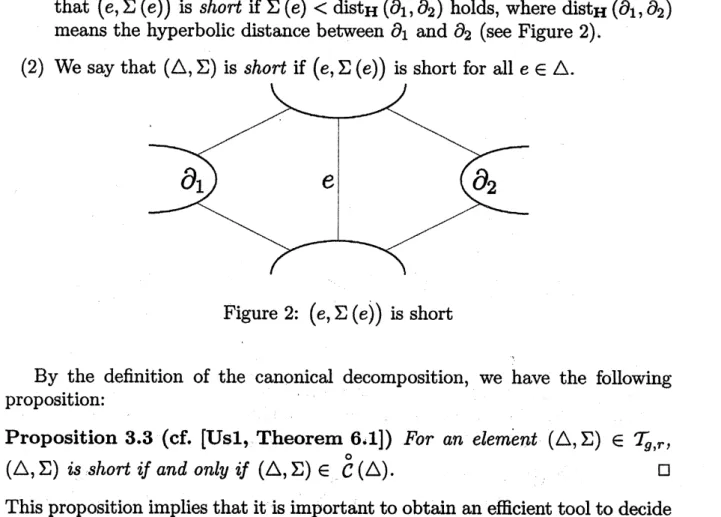
say

that $(e, \Sigma(e))$ is short if$\Sigma(e)<\mathrm{d}\mathrm{i}\mathrm{s}\mathrm{t}_{\mathrm{H}}(\partial_{1}, \partial_{2})$ holds, where $\mathrm{d}\mathrm{i}\mathrm{s}\mathrm{t}_{\mathrm{H}}(\partial_{1}, \partial_{2})$

means

the hyperbolic distance between $\partial_{1}$ and $\partial_{2}$ (see Figure 2).

Figure 2: $(e, \Sigma(e))$ is short

By the definition of the $\mathrm{c}\mathrm{a}\mathrm{n}\mathrm{o}\mathrm{n}\mathrm{i}_{\mathrm{C}\mathrm{a}}.1$ decomposition,

we

have the following

proposition:

Proposition 3.3 (cf. [Usl, Theorem 6:1]) For

an

eleme$nt(\triangle, \Sigma)\in T_{g,r}$,

$(\triangle, \Sigma)$ is short

if

and only

if

$(\triangle, \Sigma)\in$

. $C\circ(\triangle)$

.

$\square$

This proposition implies that it is important

to

obtain

an

efficient toolto decide the given

arc

is

short

or

not, and the following $h$-length coordinate is the

one.

3.2

$h$

-length

coordinate

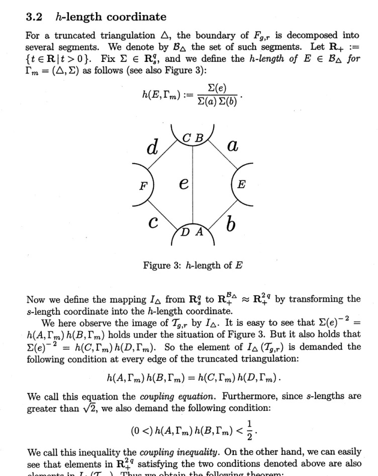
For a truncated triangulation $\triangle$, the boundary of

$F_{g,r}$ is decomposed into

several segments. We denote by $B_{\triangle}$ the set of such segments. Let $\mathrm{R}_{+}$ _$:=$

$\{t\in \mathrm{R}|t>0\}$

.

Fix $\Sigma\in \mathrm{R}_{s}^{q}$, and

we

define the $h$-length

of

$E\in B_{\triangle}$

for

$\Gamma_{m}=(\triangle, \Sigma)$

as

follows (see also Figure 3):

$h(E, \Gamma_{m}):=\frac{\Sigma(e)}{\Sigma(a)\Sigma(b)}$

.

Figure 3: $h$-length of $E$

Now

we

define the mapping $I_{\triangle}$ from $\mathrm{R}_{s}^{q}$ to $\mathrm{R}_{+}^{B_{\Delta}}\approx \mathrm{R}_{+}^{2q}$ by transforming the

$s$-length coordinate into the $h$-length coordinate.

We here observe the image of $\mathcal{T}_{g,r}$ by $I_{\triangle}$. It is easy to

see

that $\Sigma(e)^{-2}=$

$h(A, \Gamma_{m})h(B, \Gamma m)$ holds under the situation of Figure 3. But it also holds that

$\Sigma(e)^{-2}=h(C, \Gamma m)h(D, \Gamma m)$

.

So the element of $I_{\triangle}(\mathcal{T}_{g_{)}r})$ is demanded the

following condition at every edge of the truncated triangulation:

$h(A, \Gamma_{m})h(B, \Gamma m)=h(C, \Gamma_{m})h(D, \Gamma m)$

.

We call this equation the coupling equation. Furthermore, since $s$-lengths

are

greater than $\sqrt{\mathit{2}}$, we also demand the following condition:

$(0<)h(A, \Gamma m)h(B,\Gamma m)<\frac{1}{\mathit{2}}$

.

We callthis inequality the coupling inequality. On the other hand, we

can

easily

see

that elements in $\mathrm{R}_{+}^{2q}$ satisfying the two conditions denoted above

are

also

elements in $I_{\triangle}(\mathcal{T}_{g,r})$

.

Thus we obtain the following theorem:

Theorem 3.4 ($[\mathrm{U}\mathrm{s}1$

,

Proposition 4.4]) The mapping $I_{\triangle}$ is

an

embedding

of

$\mathcal{T}_{g,r}$ into

$\mathrm{R}_{+}^{B_{\Delta}}$ Explicitly, $I_{\triangle}(\tau_{\mathit{9}},r)\subset \mathrm{R}_{+}^{B_{\Delta}}$ is characterized by the

$couplin_{\square }g$

Using the $h$-length coordinate,

we

can

easily

see

whether the given edge is

short

or

not.

Proposition 3.5 ($[\mathrm{U}\mathrm{s}1$

,

Theorem 6.1]) Under the situation

of

Figure 3,

$(e, \Sigma(e))$ is short

if

and only

if

the inequality

$h(A,\Gamma_{m})+h(B,\Gamma_{m})+h(c,\Gamma_{m})+\square$

$h(D,\Gamma_{m})>h(E,\Gamma_{m})+h(F, \Gamma_{m})$ holds.

Note

We

can

extend Proposition

3.5

to the following

one:

Proposition 3.6 Under the situation

_of

Figure $\mathit{3}_{f}\Sigma(e)=\mathrm{d}\mathrm{i}\mathrm{s}\mathrm{t}_{\mathrm{H}}(E, F)$ (resp.

$>)$

if

and only

if

$h(A,\Gamma_{m})+h(B, \Gamma_{m})+h(C, \Gamma_{m})+h(D, \Gamma_{m})=h(E, \Gamma_{m})+\square$

$h(F, \Gamma_{m})$ (resp. $<$) holds.

These two propositions

are

kinds of so-called “tilt proposition.” In [Us2],

we

study

a

generalization ofthe tilt proposition.

3.3

Changing bases

As

we saw

the preceding subsection, Though the $h$-length coordinate gives

an

effective formulato decidewhether thegiven edge is short

or

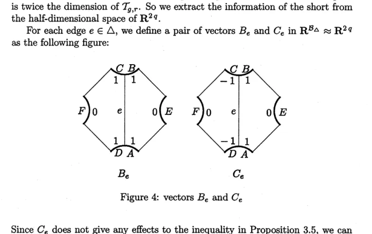
not. But the space

is twice the dimension of$\mathcal{T}_{g,r}$

.

So

we

extract the information ofthe short from

the half-dimensional space of$\mathrm{R}^{2q}$

.

For each edge $e\in\triangle$,

we

define

a

pair ofvectors $B_{e}$

and

$C_{e}$ in $\mathrm{R}^{\mathcal{B}_{\Delta}}\approx \mathrm{R}^{2q}$

as

the following figure:

$B_{e}$ $C_{e}$ Figure 4: vectors $B_{e}$ and $C_{e}$

Since $C_{e}$ does not give any effects to the inequality in Proposition 3.5,

we can

easily obtain the following proposition:

Proposition 3.7 ($[\mathrm{U}\mathrm{s}1$

,

Lemma 6.3]) (1) The set

of

vectors _{$\{B_{e}, c_{e}\}_{6}\in\triangle$}

is

a

basis

_of

$\mathrm{R}^{B_{\Delta}}\approx \mathrm{R}^{2q}$

.

Namely

(2) Suppose $I_{\triangle}(( \triangle, \Sigma))=\sum_{e\in\triangle}x_{ee}$$B+ \sum_{e\in\triangle}yeC_{e}$

for

some

$x_{e},y_{e},$

$\in$ R. Then $(\triangle, \Sigma)$ is short

if

and only

if

$x_{e}>0$

for

every $e\in\triangle$

.

$\square$

3.4

The

core

of

the

proof

We define subsets of$\mathrm{R}_{+}^{B_{\Delta}}$

as

follows:

$X^{\mathrm{o}}$

$:=$ $\{\sum_{e\in\triangle}xeBe\in \mathrm{R}_{+}^{B}\Delta$ $x_{e}>0\}$ ,

$v_{\triangle()}\circ\triangle$

$:=$ $\{z\in \mathrm{R}_{+^{\Delta}}B|\mathrm{a}\mathrm{n}\mathrm{d}(z\mathrm{s}\mathrm{a}\mathrm{t}\mathrm{i}\mathrm{s}\mathrm{f}\mathrm{i}\mathrm{e}\mathrm{S}\triangle, I^{-}1(_{Z}\triangle)\mathrm{t}\mathrm{h}\mathrm{e}\mathrm{C}\mathrm{o})\mathrm{i}\mathrm{s}\mathrm{s}\mathrm{t}\mathrm{u}\mathrm{p}1\mathrm{i}\mathrm{n}_{\mathrm{h}}\mathrm{g}_{\mathrm{o}\mathrm{r}}\mathrm{e}\mathrm{q}\mathrm{u}\mathrm{a}\mathrm{t}\mathrm{i}\mathrm{o}\mathrm{n}\mathrm{S},$ $\}$ ,

$g_{\triangle}\circ(\triangle)$

$:=$ $\{z\in D\mathrm{o}_{\triangle}(\triangle)|z$ satisfies the coupling $\mathrm{i}\mathrm{n}\mathrm{e}\mathrm{q}\mathrm{u}\mathrm{a}\mathrm{l}\mathrm{i}\mathrm{t}\mathrm{i}\mathrm{e}\mathrm{s}\}$

We note that $I_{\triangle}\circ S_{\triangle}(C(\circ\triangle))=\mathcal{G}_{\triangle}\circ(\triangle)$ by

an

immediate consequence of

Theo-rem

3.1, Proposition 3.3 and Theorem 3.4.

Now the following theorem holds:

Theorem 3.8 ($[\mathrm{U}\mathrm{s}1$

,

Theorem 6.4]

or

[Pe, Theorem 5.4]) The projection

$\Pi_{\triangle}$ induces

a

homeomorphism

from

$D_{\triangle}\circ(\triangle)$

to $x^{\mathrm{o}}$

.

$\square$

By the definition ofthe coupling inequality,

we

can

easilyprove that $\mathcal{G}_{\triangle}\circ(\triangle)$

is homeomorphic to the intersection of$D\mathrm{o}_{\triangle}(\triangle)$

and the open unit ball in $\mathrm{R}^{B_{\Delta}}$

centered at the origin. Thus

we

obtain the following theorem, which is the goal

of this section:

Theorem 3.9 ($[\mathrm{U}\mathrm{s}1$

,

Theorem 6.5]) The set $C\circ(\triangle)$ is $h_{omeom}o\mathit{7}phiC$ to $an\square$

open ball

_of

dimension $q=\mathit{6}g-\mathit{6}+3r$

.

A

Examples

Example

1.

$\mathcal{T}_{0,3}$

$x:= \sqrt{2}\cosh\frac{d_{X}}{\mathit{2}}$ ,

$y:= \sqrt{\mathit{2}}\cosh\frac{d_{Y}}{\mathit{2}}$ ,

Example

2.

$\mathcal{T}_{1,1}$

$x:= \sqrt{2}\cosh\frac{d_{X}}{2}$ ,

$y:= \sqrt{2}\cosh\frac{d_{Y}}{\mathit{2}}$ ,

$[egg1]$ $[egg2]$ $[egg3]$ $[egg4]$ $[egg5]$ $[egg6]$ $[egg7]$ $[egg8]$ $[egg9]$ _{${ }$}

References

[EP] D. B. A. Epstein and R. C. Penner, Euclidean decompositions

_of

non-compact hyperbolic manifolds, Journal ofDifferential Geometry 27 (1988),

67-80.

[Ko] Sadayoshi Kojima, Polyhedral decomposition

_of

hyperbolic

_manifolds

with

boundary, On the Geometric Structure of Manifolds, edited by Dong Pyo Chi, Proceedings of Workshops in Pure Mathematics, Volume 10, Part III (1990),

37-57.

[N\"a] Marjatta N\"a\"at\"anen, A cellularparameterization

_for

dosed

_surfaces

with

a

distinguished point, Annales

Academiae

Scientiarum Fennicae Series A. I.

Mathematica 18 (1993),

45-64.

[NN] Toshihiro Nakanishi and Marjatta N\"a\"at\"anen, The Teichm\"uller space

_of

a

punctured

_surface

represented

as a

real algebraic space, Michigan

Mathe-matical Journal 42 (1995),

235-258.

[NP] M. N\"a\"at\"anen and R. C. Penner, The

convex

hull construction

_for

compact

surfaces

and the Dirichlet polygon, Bulletin of the London Mathematical Society 23 (1991), 568-574.

[Pe] R. C. Penner, The decorated Teichm\"ullerspace

_of

punctured surfaces,

Com-munications in Mathematical Physics 113 (1987), 299-339.

[Ra] John G. Ratcliffe, Foundations

_of

Hyperbolic Manifolds, Graduate Texts

of Mathematics, 149, Springer-Verlag, 1994.

[Th] William P. Thurston, Three Dimensional

_Geometw

and Topology,

Prince-ton Mathematical Series, 35, Princeton University Press, 1997.

[Usl] Akira Ushijima,

A

canonical cellular decomposition

_of

the Teichm\"uller

space

_of

compact

_surfaces

with boundary, Communications inMathematical

Physics 201 (1999), 305-326.

[Us2] Akira Ushijima, The tilt

_formula

_for

weighted simplices in hyperbolic