Some Mathematical Considerations on Parent-Offspring Conflict Phenomenon(Mathematical Topics in Biology)

(1)

227 Some

Mathematical

Considerations

on Parent-Offspring

Conflict

Phenomenon

Hiromi

SENO

and Hiroki

TOKUDA

Department

_of

Mathematics, Faculty

_of

Science, _Hiroshima University

子の独立時期についての親子間衝突に関する数理モデル解析

瀬野裕美・徳田博樹

広島大学理学部

Astochastic dynamicprogramming model for

parent-offspring confictisanalyzed anddiscussed. Itisdiscussed

how the confiict is resolved and how the ultilllate

off-spring’s independence age is determined between parent

and offspring. Results by the mathematical model

in-dicates such possibility that the observed behaviour of

parentalcare may ch ange depending on the parent’sage.

Thisisbecause the compromise conclusion of the

parent-offspring conflict depends on the parent’s age, that is

essentially, on the parent’s expected futurereproductive

value. Moreover, it is shown that the observed

parent-offspring confbct possibly depends on the parent’s age, too.

INTRODUCTION

In behavioural ecology, many researchers have

been interested in and have discussed the

parent-offspring conflict phenomenon: offspring wantsto

become independent ofparent and to feed by

it-self after an age$t_{o},$ $w1_{1}ile$parentofits age$a$ wants

tostopfeeding after an offspring’s age $t_{p}(a)$. The

critical day $t_{p}(a)$ from the parent’s viewpoint is

assumed to depend on theparent’s age $a$

.

When

$t_{o}$ and $t_{p}(a)$ do not coincide with each other, a

conflict takes place between parent and offspring.

Thereare possiblytwodifferenttypesof such

con-flict: $t_{o}^{l}<t_{p}(a);t_{o}>t_{p}^{l}(a)$

.

Under the conflict in

the case when $t_{o}<t_{p}(a)$, offspring wants to

be-come independent of parent, while parent wants

to feed offspring. On the other hand,in the case

when $t_{o}>t_{p}(a)$, offspring wants to befed, while

parent wants to stop feeding. Only when $t_{o}=$

$t_{p}(a)$, any conflict doesn’t take place. However,

since $t_{o}$ does not depend on the parent’s age $a$,

whereas $t_{p}(a)$ does, the conflict between parent

and offspringisobservable very much.

In thiswork,we analyze astochasticdynamic

pro-gramming model which corresponds tothe model

constructed by Clark and Ydenberg (1990). In

our model, differently from their model, parentis

assumed to have a finite reproducible age-span,

so that its future reproductive value is explicitly

variable depending on the parent’s age. A

spe-cificgrowthfunctionand a specific terminal fitness

function areintroduced. Analyzing themodel,we

discuss the characteristics of the optimal critical

ages$t_{o}$and$t_{p}(a)$, anditis shown that possibly

ex-istentconflictisonly thetype that $t_{o}>t_{p}(a)$,

in-dependently ofthe parent’sage and the other

pa-rameterscharacterizing the relation between

par-ent and offspring. Further, we discuss how the

conflict is resolved and how tbe ultimate

indepen-dence age isdetermined between parent and

off-spring.

MODEL

Parent’s and Offsprrng’s

Ages

Let $a$ denote the parent’s age, for instance, in

year, where $a_{f}\leq a\leq a_{1}$

.

$a_{f}$ and $a_{1}$ are

respec-tively the first and the last ages for the parent’s

(2)

$”’$

$\infty aen$ $\sim_{s}$

$\vdash’’+^{\prime d\text{下_{}-}sa\underline{fter0\Uparrow}\underline{sbi}rt\text{加^{}\backslash }\backslash }\infty’\div-\infty^{\backslash }\{""\prime y_{-}sp\dot{n}n_{9_{-}’\backslash }\backslash \backslash \backslash \backslash$

12 $t_{l}$ r-l $T$

$-hnnt*\prime c_{n}\text{\’{e}} n(o_{f},\sigma)arrow 2^{o\kappa_{\epsilon m\eta\dot{\}}}j_{nm_{\sigma_{r}^{n}}\infty_{\sigma_{o})}}$

(

Fig.1. Modelling the parent-offspringrelauon.

reproduction. Hence, the reproducible age-span

for every parent is given by $a\iota-a_{f}+1$. The

off-spring’s age in day during a breeding season is

denoted by $t$,where _{$1\leq t\leq T$}. $T$is the length in

dayofbreeding season (seeFig. 1).

Offsp7ring$s$

Growth

We use the following specific growth function

foroffspring:

$Y(t+1)=\{Y(t)+Y(t)+k_{t=t,t_{S}+1^{s},..,T-1}fort^{1}=1_{s}2,\ldots,t-.1r\circ r^{k_{2}}(I)$

$Y(1)=Y_{1}$, (2)

that is,

$Y(t)=\{\begin{array}{l}k_{1}(t-1)+Y_{1}k_{2}(t\frac{}{f}t_{S})+k_{s^{1}}(t_{\delta}-1)+Y_{1}r_{ort=1,2_{\prime}}ort=t+1_{\prime}t^{t_{s^{S}}}+2,\ldots,T\end{array}$ (3)

where$Y(t)$ is the offspring’s weight at the

begin-ning of day$t$,and $Y_{1}$ is the offspring’s weight at its

birth. $t_{s}$ is theoffspring’s age when parent stops

. _{feeding and offspring becomes} _independent. $k_{1}$ is

a positive constant which means the offspring’s

daily growth rate with the parent’s feeding, while

$k_{2}$ is a positive constant which means the

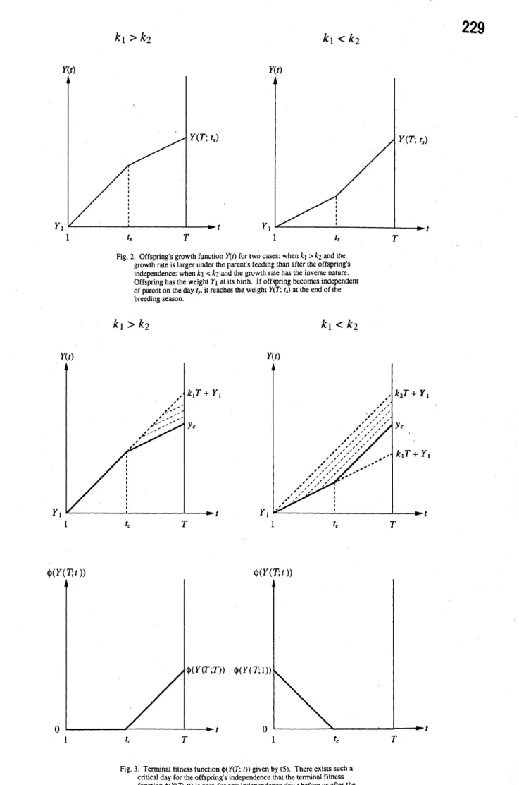
inde-pendent offspring’s daily growth rate(see Fig. 2).

Now, consider the offspring’s weight$Y(T;t_{s})$ at

the beginning of thelast day$T$of thebreeding

sea-son, under the condition that offspring becomes

independent at day $t_{s}$. From (3), $Y(T;t_{s})$ is

ex-pressed as follows:

$Y(T, t_{\theta})=k_{2}(T-t_{S})+k_{1}(t_{S}-1)+Y_{1}$. (4)

Offspring’s

Fitness

We define thedaily survival probability $\sigma_{n}$ for

offspring fed by parent, the daily survival

proba-bility $\sigma_{o}$ for offspring independent ofparent, the

daily survivalprobability $\sigma_{f}$forparentfeeding

off-spring, and the daily survival probability $\sigma_{p}$ for

parent not feeding offspring (see Fig. 1). As

Ydenberg (1989) showed in general for alcids, it

is naturally assumed that $\sigma_{o}<\sigma_{n}$ and $\sigma_{f}<\sigma_{p}$

.

The following events significant to determine the

offspring’s fitness are assumed on each day: (i)

Ifparent survives and feeds offspring with

prob-ability $\sigma_{f}$, offspring grows following to (3) with

its survival probability $\sigma_{n}$; (ii)$|If$parent dies with

probability $1-\sigma_{f}$,offspring becomes independent

togrow followingto (3)withits survival

probabil-ity $\sigma_{o}$; (iii) Ifparent stops feeding offspring with

its survival probability$\sigma_{p}$,offspring becomes

inde-pendent togrow following to (3) with its survival

probability$\sigma_{o}$.

Consider such probability $\phi(1^{\prime’}(T;t_{\dot{\theta}}))$ that

off-spring $wit1_{1}$ weight _{$Y(T;t_{s})$} at the end of the

breeding season will survive

_after

thebreeding

sea-son and reach thereproducible age to reproduce

the next generation. The probability $\phi(Y(T;t_{s}))$

is called the terminal

_{fitness function}

foroffspring,

andgiven as follows:

$\phi(1’(T;t_{s}))=\{$ $\gamma(YT\cdot t)0oth’erwise^{y}!t_{S})>y_{C};(5)$

where $\gamma$is a positiveconstant translating the

ad-vantage ofweight gain $Y(T;t_{s})-y_{C}$ to the

prob-ability $\phi(Y(T;t_{S}))$

.

$y_{C}$ is theoffspring’s minimum

body weight at the end of the breeding season,

sufficient tosurvive

_after

thebreeding season and

reach its reproducible age to reproduce the next

generation (seeFig. 3).

Conventionally, we define the critical day $t_{c}$

such that $Y(T;t_{c})=y_{c}$, which is given by

$t_{c} \equiv\frac{y_{C}-Y_{1}+k_{1}-k_{2}T}{k_{1}-k_{2}}$. (6)

Used the notation $t_{c}$, the probability $\phi(Y(T;t_{s}))$

can beexpressed in thefollowing way:

When $k_{1}>k_{2}$,

$\phi(Y(T;t_{s}))=\{\begin{array}{l}\gamma(k_{1}-k_{2})(t_{s}ift_{S}>^{-}t^{t_{c^{c}}.,)}0otherwise\end{array}$ (7)

When $k_{1}<k_{2}$,

(8)

$\phi(Y(\mathcal{T};t_{\delta}))=\{\begin{array}{l}\gamma(k_{2}-k_{1})(t_{c}if\ell_{S}<^{-}\ell^{\iota_{c^{s}}.)}0otherwise\end{array}$

Eventually, it is assumed that $1<t_{c}<T$. In the

case when$k_{1}>k_{2}$, iftheoffspring’sindependence

day$t_{s}$ is earlier than the critical day$[t_{c}]+1$ given

by (6), theoffspring’s weight $Y(T;t,)$ at the end

of the breeding season is below$y_{c}$so that the

ter-minal fitness function $\phi(Y(T;t_{s})$ is zero (Fig. 3).

In contrast, in the case when $k_{1}<k_{2}$, ifthe

off-spring’s independence day $t_{s}$is later than $[t_{c}]$,the

terminal fitness function $\phi(Y(T;t_{s})$ is zero.

Now, we consider the offspring’s fitness $F_{o}(t_{s})$

defined as such probability that offspring can

sur-vive through and

after

the breeding season and

(3)

$k_{1}>k_{2}$ $k_{1}<k_{2}$

Fig.2. Offspring’s growth function$Y(t)$fortwocases:when$k_{1}>k?\sim$and the

growthrateis larger under the parent’s feeding than after the offspring’s

independence; when$k_{1}<k_{2}$andthe growth rate has the inverse nature.

Offspring hastheweight$Y_{1}$atits birth. lf offspnng becomes independent

ofparentontheday$t_{S}$

.

itreaches the weight$Y(T;t_{s})$atthe endofthe

breedingseason.

$k_{1}>k_{2}$ $k_{1}<k_{2}$

Fig.3. Terrmnalfitness function$\phi(Y(T;t))$given by(5). Thereexists sucha

cnuca! day fortheoffspnng’s independencethat theterminalfitness

function$\phi(Y(T;t))$iszerotoranyindependence day$t$beforeorafterthe

(4)

generation, under the condition that it becomes

independent on day $t_{S}$ of the breeding season. If

offspring becomes independent on the first day,

that is, $t_{s}=1$, it survives through the breeding

season with probability $\sigma_{o}^{T}$. Growingupwith (3),

the offspring’s weight reaches $Y(T;1)$ at the last

day $T$of thebreeding season, which means that,

after

thebreedingseason,offspring gets the

prob-ability $\phi(Y(T;1))$ to survive and reach its

repro-ducible age. Hence, the offspring’s fitness $F_{o}(1)$ is

given by

$F_{o}(1)=\sigma_{o}^{T}\phi(Y(T;1))$_. ₍₉₎

In the case when $t_{s}=2$, two cases arise to be

considered. The first case isthat,ifparentdies on

the first day with probability $1-\sigma_{f}$, offspring is

i

糖鍛鰯響鞭

\not\in n

漉難窺難

$pt$

嚇

hernepet

撫

ability $\sigma_{o}^{T}$

.

Therefore, the fitness in this case is

given by$F_{o}(1)$with probability $1-\sigma_{f}$. Thesecond

詳諸認織雅

r

認撒響

fd, 講

r

離播

and survives for oneday with probability $\sigma_{n}$

.

For

$o^{s}n\overline{\overline{d}}d^{\sim}t_{therest\circ fthebreedingseason^{ri_{W1}survives}}^{0ffs}Tl9throug^{a}f_{en,theindependentoffspng_{thproba-}}^{ri\iota\iota gbecomesindependentonthe\sec-}$

bilty$\sigma_{O}^{T-1}$

.

Theoffspring‘sweight reaches$Y(T;2)$

on day $T$, which means that,

after

the breeding

season, offspring gets the probability $\phi(Y(T;2))$

to survive and reachits reproducible age. Lastly,

the offsping’sfitness $F_{o}(2)$ isgiven by

$F_{O}(2)=$($1$–a

$f$)$\sigma_{O}^{T}\phi(Y(T;1))$

(10)

$+\sigma_{f}\sigma_{n}\sigma_{o}^{T-1}\phi(Y(’\Gamma;^{o}\sim))$.

In the case when $t_{s}=3$, three cases arise. The

first case is that parentdies on the first day with

probability $1-\sigma_{f}$. Thesecondcase is that parent

survives on the first day with probability $\sigma_{f}$ and

dies on the second daywith probability $1-\sigma_{f}$. In

this case from the second day, offspring becomes

$independ_{en}t$ _{and survives through the rest of the}

$Caseisb\circ thofbreedin_{t}fi_{th^{a}e}^{se_{t}asonwithprobabi1ity_{feedsoffs}}\not\in arentsurvivesandf_{proba-}^{ringon}$

$T-1$_. _{The third}

bility $\sigma_{f}^{2}$

.

In this case, offspringsurvives for two

days with probability $\sigma_{n}^{2}$. For $t_{s}=3$, offspring

becomes independent on the third day. The

mde-pendent offspring survives through the rest of the

breeding season with probability$\sigma_{o}^{T-2}$. Lastly,the

offspring’s fitness$F_{o}(3)$ is givenby

$F_{o}(3)=(1-\sigma_{f})\sigma_{o}^{T}\phi(Y(T;1))$

$+\sigma_{f}(1-\sigma_{f})\sigma_{n}\sigma_{o}^{T-1}\phi(Y(T;2))$ (11) $+\sigma_{f}^{2}\sigma_{n}^{2}a_{o}^{T-2}\phi(Y(T;3))$.

For the case when $t_{s}=4,5,$$\ldots,$$T,$$F_{o}(t_{s})$is given

in the sameway.

Consequently, except for the case when $t_{s}=$

$1,$ $F_{o}(t_{s})$ is expressedin general as follows:

$F_{O} \langle l,)=\sum_{j=1}^{t_{*}-1}\sigma_{f}^{j-1}\langle 1-\sigma_{j})\sigma_{\mathfrak{n}}^{j-1}\sigma_{O}^{T-j+1}\phi(Y^{-}(T:j))$

$+\sigma_{j}^{1-1}\sigma_{n^{l}}^{l-1}\sigma_{o}^{T-t_{9}+1}\phi(Y(T;\ell_{i}))$.

(12)

Parent’s

Survival

Probability

In this section, We consider the parent’s

sur-vival probability $F_{p}(t_{s})$, which is defined as

such probability thatparentsurvives through the

breeding season under the condition that it stops

feeding on day$t_{s}$in the breeding season. Now, $\sigma_{w}$

is defined assuch probability that parentsurvives

through the interval period between two sequent

breeding seasons and reaches the next breeding

season.

If parent never feeds offspring on any day

through the breeding season, that is, if $t_{S}=1$,

parentsurvives through the breeding season with

probability $\sigma_{p}^{T}$. Then, parent can reach the next

breedingseason with probability $\sigma_{w}$

.

Hence, the

parent’ssurvival probability $F_{p}(1)$ is given by

$F_{P}(1)=\sigma_{p}^{T}\sigma_{w}$. (13)

Ifparent feeds offspring on the first day and

stopsfeeding on the second day, that is, if$t_{s}=2$,

parent survives on the first day with probability

$\sigma_{f}$ and through the rest of the breeding season

with probability $\sigma_{p}^{T-1}$

.

Hence, the parent’s

sur-vival probability $F_{p}(2)$ isgiven by

$F_{p}(2)=a_{f}a_{p}^{T-1}\sigma_{w}$. (14)

In the case when $t_{s}=3$, two cases arise to be

considered. The first case is that parent feeds

off-springon the first day with its survival probability

$\sigma_{f}$,while offspring dies on the first day with

prob-ability $1-\sigma_{n}$. Then, parentsurvives through the

restofthebreedingseason with probability$\sigma_{p}^{T-1}$.

The second case is thatparent feeds offspring on

the firstdaywithits survival probability$\sigma_{f}$,while

offspring survives on the secondday with its

sur-vival probability $\sigma_{n}$

.

Parent feeds offspring also

on the second day with its survival probability

$\sigma_{f}$

.

For $t_{s}=3$, parent stops feeding on the third

day. Then, parentsurvives through the rest of the

breeding season with probability$\sigma_{p}^{T-2}$. Lastly, the

(5)

$F_{p}(3)=\{(1-\sigma_{n})a_{f}\sigma_{p}^{T-}+a_{n}a_{f}^{2}\sigma_{p}^{T-2}\}\sigma_{w}.(15)$

For the case when $t_{S}=4,5,$$\ldots,$$T,$$F_{p}(t_{s})$ is given

in thesame $wav$.

Consequently, except for the case when $t_{s}=1$

or$t_{s}=2,$ $F_{p}(t_{s})$is expressed in general as follows:

$F_{p}(t_{s})$ $=a_{w} \sum_{j=1}^{t,-2}\sigma_{n}^{j-1}(1-a_{n})\sigma_{f}^{j}a_{p}^{T-j}$

(16)

$+a_{w}\sigma_{n}^{t.-2}\sigma_{f}^{t.-1}\sigma_{p}^{T-\iota.+1}$.

reproductive value $R(a_{1}-1)$ for the age$a\iota-1$ is

determined by

$R(a_{l}-I)$ $=$ $\sigma_{w}J(t_{p}(a_{\iota});R(a_{\iota}))$

$=$ $a_{w}F_{O}(i_{p}(a_{\iota}))$, (19)

and, further, in general, the value $R(a_{l}-i)(i=$

$1,2,$$\ldots,$$a\iota$ –a

$’$) for the age $a\iota-i$is given by the

following backwardrecurrence equation:

$R(a_{\iota}-i)=\sigma_{w}J(t_{p}(a_{\iota}-i+1);R(a_{l}-i+1)).(20)$

MODEL Parent’s Fitness

Consider the parent’s fitness atits age$a$, under

thecondition thatitstopsfeeding on day$t_{s}$ of the

breeding season. The parent’s fitness $J(t_{s}; R(a))$

is defined by the parent’s survival probability

$F_{p}(t_{s})$, its offspring’s fitness $F_{o}(t_{s})$, and the

par-ent’s expected future reproductive value $R(a)$ at

thelast day of the breeding season at the parent’s

age$a$, which satisfies thefollowing:

$R(a)=a_{w}J(t_{S}; R(a+1))$

(17)

$(a=a_{f}, a_{f}+1, \ldots, a_{\iota}-1)^{-}$

$J(t_{s} ; R(a+1))$ means the parent’s fitness at its

age $a+1$

.

Since $\sigma_{w}$ means the probability that

parent survives between the end of the breeding

season at its age$a$ and thebeginning of the next

breeding season atits age$a+1$,therighthandside

of (17) means the expected future reproductive

value. Remark that$R(a)$should be monotonically

decreasing in terms of the age $a$, and $R(a\iota)=0$

because $a_{l}$ is the last age for the parent’s

repro-duction.

As in Clark and Ydenberg (1990), $J(t_{s}; R(a))$

isgiven in this paper as follows:

$J(t_{S} ; R(a))=F_{O}(t_{S})+R(a)F_{p}(t_{S})$. (18)

From (17)and (18),wecan obtain the backward

recurrenceequation todetermine the expected

fu-ture reproductive value $R(a)$ for every age $a$

.

It

is assumed that, since the expected future

repro-ductive value$R(a)$is considered only forparentto

determine its behaviour$t_{p}(a)$ from its viewpoint,

it has no relationwith$t_{o}$from the offspring’s

view-point. Thus, since $R(a_{\iota})=0$, the expected future

ANALYSIS

The Optimal

Offsp

ring$s$ Independence

Age

From The

Offspring’s

Viewpoint

The $opt_{!}md$ offspring’s independence age $t_{o}$

from offspring’s $viewp_{01}nt$ is defined as the day

to maximize the offspring’s fitness $F_{o}(t_{s})$ in the

breeding season. Therefore, by analyzing $F_{o}(t_{s})$

givenby (9) and (12) (as for the way of analysis,

see Appendix A), $t_{o}$ can be obtained as follows

(Fig. 4): When $k_{1}>k_{2}$, $\ell_{O}=T$. (21) When $k_{1}<k_{2}$, $t_{o}=\{\begin{array}{l}n1ift<\nu+if\nu^{c}+n<t_{c\leq}^{2}\nu+n+1(n=2,3,\ldots\prime T-1)\end{array}$ (22) where $\nu\equiv\frac{1}{\sigma_{n}/\sigma_{O}-1}$. (23)

Since $\sigma_{n}>\sigma_{o}$ from the assumption, $0<\nu<\infty$

.

For convenience, we will hereafter use thenotation

$\nu$

.

As seen in Fig. 4, those conditions for$t_{o}$in the

case when $k_{1}<k_{2}$,givenby (22), are

complemen-taryeach $otl\iota er$, and the possibly maximal $F_{o}(t_{s})$

is$T-1$ in the case.

The

Optimal Offspring’s Independence Age

From Parent’s Viewpoint

Theoptimaloffspring’s independence age$t_{p}^{l}(a)$

from the parent’s viewpoint is defined as the

off-spring’s age $t_{s}|$ to maximize the parent’s fitness

(6)

Fig. 4. Inthecasewhen$k_{1}<k_{2}$,theoptimal offspnng’s independenceage$t_{o^{*}}$

fromtheoffspnng’sviewpointontheparameterspace$(V, t_{c})$. For$1<t_{c}<$

$T,$ $t_{o}^{*}<T$.

Fig.5. In thecasewhen$k_{1}>k_{2}$,the parameterspace$(p. K(n))$iscategorized

into$I_{1}-I_{7}$,dependingonthe typeotthe division of the parameterspace $(v, t_{c})$intermsof the value$0\dot{f}t_{p}^{*}(\iota)$.

$I_{1}$ $I_{2}$

$I_{3}$ $L$

Fig. 6. $\ln$thecasewhen$k_{1}>k_{2}$,theoptimaloftspring$s$independence,Igc

$t_{p}^{*}(a)$from the parent’sviewpointonthe$pu\phi met_{C^{\backslash }}r$space$(v, t\cdot)$forthe

parameter sets$I_{1}-I_{4}$of theparameterspace$(p, K(\iota))$.

Fig.7. In thecasewhen$k_{1}>k_{2}$,the optimal offspring’sindependenceage $t_{p^{*}}(a)$fromthe parent’sviewpointonthe parameterspace$(v, t_{c})$torthe

(7)

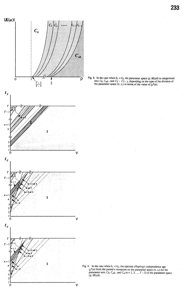
Fig.8. In thecasewhen$k_{1}<k_{2}$,theparameterspace$(p, \mathfrak{l}K(a)1)$is categonzed

into$C0$

.

$C_{dt}$_,and$C_{2}\sim Cr-2$_,_dependingon_the_{type of}_the_{division of}

the parameterspace$(v, t_{c})$intermsof the value of$t_{p^{*}}(a)$.

Fig.9. Inthecasewhen$k_{l}<k_{2}$,theoptimaloffspnng’s independenceage

$t_{P^{*}}(a)$fromthe parent’sviewpointonthe parameterspace$(v, t_{c})$for the

parametersets,$C_{0},$$C_{all}$_,and_{$C_{n}(n=2,3, \ldots, T-2)$}ofthe_parameterspace

(8)

(18), $t_{p}(a)$ can be obtained for the parent’s age

$a$, when $R(a)>0$,that is, when a$f\leq a\leq a_{\iota}-1$,

as follows: When $k_{1}>k_{2}$,

$t_{p}(a)=\{Tlni^{i\leq_{+_{\ell}^{t<}}^{(\nu_{C}\cdot a\rangle_{(\nu\cdot.\alpha_{\circ)}}}}i_{ T\leq_{T\frac{9}{h}}}i^{ft>_{(n_{l}=}}orilt<^{2}orii\ell<_{\mathfrak{n}+_{2^{l_{\prime}}}^{n^{l_{\frac{\{}{ct_{3}}}}}}^{n}n_{an_{d^{c^{l}}h_{C}\nu.a.)\leq t_{C}<h_{n}\langle\nu.\alpha)}}^{c}an_{-}^{d_{C}h^{g}\nu\cdot...a_{\nu}).\leq.l_{C}<.g_{\mathfrak{n}}\{\nu\cdot..a\rangle}and\ell c<r^{<_{l}\tau^{T_{)}-l)}}an^{-}d\ell<\tau^{l}t^{n}’$ (24)

When $k_{1}<k_{2}$,

$t_{p}(a)=\{n1i^{ft<h(\nu.\cdot a)}i_{fh^{c_{n}}(\nu\cdot.a)<t_{c}..\leq h_{n+}(n=^{1}2,3,.,T-1^{1})^{(\nu\cdot.a)}}$ (25) where

$g_{n}( \nu;a)\equiv n+\frac{\rho^{T-n+2}\nu}{K(a)\nu+1}$ (26)

$h_{\hslash}( \nu;a)\equiv n+(1-\frac{\rho^{T-n+2}}{K(a)})\nu$ (27)

$\rho\equiv\frac{\sigma_{p}}{\sigma_{O}}$ (28)

$K(a) \equiv\frac{\gamma(k_{1}-k_{2})\sigma_{P}/\sigma_{w}}{R(a)\sigma_{p}/\sigma_{f}-1}$. (29)

Note that those conditions for $t_{p}(a)$ are not

complementary each other. For example, in the

case when $k_{1}>k_{2},$ there exist such parameters

that$g_{2}(\nu;a)<t_{c}<h_{T}(\nu;a)<T-1$

.

Thismeans

that, with such parameters, $t_{p}^{l}(a)$ should be 1 or

$T$

.

In this case, $t_{p}(a)$ can be ultimately

deter-mined by comparing $J(1;R(a))$ with $J(T;R(a))$

.

In this paper, avoiding a mess of calculations, we

no longer discuss the ultimately determined$t_{p}(a)$

insuch case, because our presented analysesgive

sufficiently significant qualitative results valuable for the discussion on the parent-offspring conflict phenomenon.

As indicatedbythoseconditions for$t_{p}(a)$,given

by (24)and (25), theultimately determined$t_{p}(a)$

strongly depends on parameters (Fig. 6, Fig. 7,

Fig. 9). The parameter space $(\nu, t_{c})$ can be

de-vided into some subregions depending on what

value is possiblefor $t_{p}(a)$. The way of the

devi-sion depends on the otherparameters$\rho$and $K(a)$

(Fig. 5, Fig. 8).

In the case when $k_{1}>k_{2}$, depending on the

$Wtecateg\circ rizetheparemeterreg\circ 7_{\iota\circ f(\rho,K(a^{c})^{)})}^{rspace(\nu,t}$

into thoseregions $I_{1}\sim I_{7}$ as shown iu Fig. 5 (as

for theanalyzingway,see AppendixB).According

tothoseparametersubregions of$(\rho, I(a))$,the

ul-timatelydetermined $t_{p}(a)$is shownin the

param-eter space $(\nu, t_{c})$ as in Fig. 6 and Fig. 7. In cases

of$I_{1},$ $I_{2}$, and $I_{4}$, the possible value of $t_{p}(a\rangle$ is $T$

or less than an $N$, while, in case of$I_{3}$, it is any

value from 1 to $T$

.

In cases of$I_{5}\sim I_{7}$, only 1 or

$T$ispossiblefor _{$t_{p}(a)$}.

In contrast, in thecase when $k_{1}<k_{2}$, we

cat-egorize the paremeter region of $(\rho, |K(a)|)$ into

thoseregions $C_{0},$$C_{n}(n=2,3, \ldots, T-2)$, and$C_{a1l}$

as shown in Fig. 8 (Appendix B). For those

re-gions, the ultimately determined$t_{p}(a)$ is shown in

the parameterspace$(\nu, t_{c})$ asin Fig. 9.

Indepen-dently of which caseisconsidered, any value from

1 to $T-1$ is possible for$t_{p}(a)$.

When $a=a_{1}$, since $R(a_{1})=0$ from the

defini-tion, it is followed that $J(t_{s}; R(a_{t}))=J(t_{s} ; 0)=$

$F_{o}(t_{s})$

.

Therefore, $t_{p}(a_{1})=t_{o}$given by (21) and

(22), and there does not occur any conflict

be-tween parent and offspring.

The offspring’s independence age $t_{p}\sim$ to

maxi-mize the parent’s survival probability $F_{p}(t_{s})$is

al-ways 1 independently of the values ofparameters,

because $F_{o}(t_{s})$ is monotonically decreasing.

In-deed,since$a_{p}>\sigma_{f}$, for any $\downarrow s$

’

$F_{P}(t_{S}+1)-F_{P}(t_{s})$

$=\sigma_{n}^{t.-1}\sigma_{f}^{t.-1}\sigma_{p}^{T-t}(a_{f}-a_{P})\sigma_{w}<0$. (30)

From the definition (18), when parent is

suf-ficiently young and $R(a)$ is so large, it is

ex-pected that$t_{p}(a)$is near $t_{p}\sim$,because _{$J(t_{s} ; R(a))\approx$}

$R(a)F_{p}(t_{s})$

.

Indeed, asseen in Fig. 6, Fig. 7, and

Fig. 9, the parameterregion for $t_{p}(a)=t_{p}\sim=1$

is relatively larger for the smaller $|K(a)|$ than for

thelarger.

Existence

_of

Parent-Offsp$7^{\vee}ing$

Conflict

Compared Fig. 4 to Fig. 6, Fig. 7, and Fig.

9, the parent-offspring confict presents for awide

range ofparameters.

In the case when $k_{1}>k_{2}$_, as shown in Fig. 6

and Fig. 7, especially forrelativelylarge value of

$t_{c}$, the parent-offspring conflict canexist, because $t_{o}=T$. The typeof conflictis eventually for $t_{o}>$ $t_{p}(a)$, that is, underconflict, parent tendsto stop

feeding its offspring, while offspring wants to be

fed. Only forsufficiently small values of$t_{c}$ and $\nu$,

(9)

parentkeepsfeeding its offspring who wants to be fed.

As well, in the case when $k_{1}<k_{2}$, as shown

in Fig. 9, only one type of conflict, $t_{o}>t_{p}^{l}(a)$,

is possible to exist and occur. This result can

be easily proved that any slope of boundaries of

parameterregions in$(\nu, t_{c})$,givenby (27),is more

than 1.

Parent’s Age Dependence

_{of Confiict}

The optimal offspring’s independence age$t_{p}(a)$

from the parent’s viewpoint for a breeding season

is determined depending on the value of $K(a)$,

that is, of $R(a)$ as shown by the above

analy-sis. Following the definition, $|K(a)|$ is

monoton-ically increasing to infinite as the parent’s age $a$

increases, since $R(a)$monotonically decreases as$a$

increases, and reaches zero at the age$a_{\iota}$

.

There-fore, as the parent’s age increases, theparameter

point moves upinthe$par\dot{a}meter$space$(\rho, |K(a)|)$.

In the case when $k_{1}>k_{2}$ and $0<K(a)$, if

$\rho\geq 1$, as the parent’s ageincreases, the

parame-ter point $(\rho, It’(a))$ moves as$I_{5}arrow I_{6}arrow I_{7}$ in Fig.

5. Therefore, since $t_{o}=T$in this case, whenever

theconflict occurs, $t_{p}(a)=1$, and parent tends to

stopfeeding its offspring on everyday of the

breed-ingseason, while offspring wants to be fed allover

the breeding season. Otherwise, when the

con-flict does not occur, then parent keeps feeding its

offspring allover the breedingseason. Moreover,

for someparameters of $(\nu, t_{c})$, as seen in Fig. 7,

the conflict does not occur for parent older than

acritical agedetermined by the parameter $(\nu,$$t_{c}$,

while theconflict occurs for the youngerparent.

If $\rho<1$ when $k_{1}>k_{2}$, as the parent’s age

increases, theparameterpoint$(\rho, K(a))$movesup

inFig. 5 through the following order ofparameter

regions in it: $I_{5}arrow I_{1}arrow I_{2}arrow I_{3}arrow I_{4}arrow I_{7}$.

Theparameter point $(\rho, K(a))$does not pass any

region with any order inverse to thisorder. The

argument similar to that for $\rho\geq 1$ is applicable

for this case. As the parent’s age increases, $t_{p}(a)$

tends to be tlte same orto increase, therefore,it is

likely that,afteracriticalparent’sage, the conflict

does not occur and parent keeps feeding all over

the breeding season.

As mentionedbefore, at theparent’s age$a\iota$ last

in the reproducible age span, in the case when

$k_{1}>k_{2}$, the conflict does notoccur and $t_{p}(a)=$ $t_{o}=T$, so that parent keeps feeding all over the

breedingseason.

It is concluded for $tl\iota e$ case when $k_{1}>k_{2}$ that

the optimal offspring’s independence age $t_{p}(a)$

from the parent’s viewpoint stays the same or

tends to become the larger toward $T$ as the

par-ent’s age$a$ increases, and the conflict of thetype

for $t_{o}>t_{p}(a)$ disappears after a parent’s age,

then. parent keeps feeding all over the breeding

season.

On the other hand, in the case when $k_{1}<k_{2}$

and $K(a)<0$ , as the parent’s age$a$increases,the

parameter point $(\rho, |K(a)|)$ moves up in Fig. 8

through the following order of parameterregions

init: $C_{a\downarrow\iota}arrow c_{\tau-2}arrow C_{T-3}arrow\cdotsarrow C_{3}arrow C_{2}arrow$

$C_{0}$. Theparameterpoint$(\rho, |K(a)|)$does not pass

any region with any order inverse to this order.

Therefore, as seen in Fig. 9, since the conflict is

only of the type that $t_{o}^{l}>t_{p}(a)$, the conflict can

disappear after a critical age of parent for some

parametersof$(\nu, t_{c})$. For the otherparametersof $(\nu, \ell_{c})$, the conflict oftype that $t_{o}>t_{p}(a)$ occurs

through the parent’s reproducibleage-spanexcept

for the last age$a\iota$

.

In bothcases, the optimal

off-spring’sindependence age$t_{p}(a)$ from theparent’s

viewpoint staysthe same or tendsto become the

largerastheparent’sage$a$increases, as wellas in

the case when $k_{1}>k_{2}$.

Resolution

_of

Parent-Offspring

_Conflict

By the above anaiysis, it is shown that the

parent-offspring conflict possibly occurs

depend-ing on those parameters including the parent’s

age. The conflict is resolved once parent or

off-springyields toanother. In this section, we discuss

how theconflictisresolved, and how the

compro-mised day $t^{\star}(a)$ whenoffspring becomes

indepen-dent isdetermined.

For the resolution of parent-offspring conflict,

the cost for conflict is taken into account. Now,

the cost for conflict is assumed to be introduced

asthe decrease of fitness(Higashi andYamamura,

1993). That is, under the conflict, it is assumed

that offspring must pay acost $c$ to counter

par-ent, while parent must pay a cost $\alpha c$ to counter

offspring, where $c$ is monotonically increasing as

the duration of the behaviour to counter another

side per conflict, and $\alpha$ is a positiveconstant. At

the beginning of any day under the conflict

sit-uation, $c=0$ because the behaviour to counter

another side is not yet started. Those costs are

subtracted from fitnesses ofparent and offspring.

In the following, we consider the resolution of

(10)

mentioned above, for two distinct cases: $t_{o}^{r}>$

$t_{p}^{r}(a);t_{o}^{l}<t_{p}(a)$.

CASE $A:t_{o}>t_{p}(a)$

The compromised day $t^{\star}(a)$ naturally satisfies

that $t_{p}(a)\leq t^{\star}(a)\leq t_{o}$. The fitness gain $D_{p}(t;a)$

forparenton a day $t$under theconflict (expected

forthe case in whichparent wins the conflict and

succeeds in making offspring independent),

rela-tive to such fitness thatparentyielded tooffspring

in the first place and let offspring depending on the

parent’sfeeding, is now givenby

$D_{p}(t;a)=J(t;R(a))-J(i+1;R(a))-\alpha c$. (31)

On the otherhand,the fitness gain $D_{o}(t;a)$for

offspring on a day $t$under the conflict (expected

for the case in which offspring wins the conflict

and succeeds in making parent feeding), relative

to such fitness that offspring yielded to parent in

the first place and became independent, is now

givenby

$D_{o}(t_{1}\cdot a)=F_{O}(t+1;a)-F_{O}(l;a)-c$. (32)

When $t_{p}(a)\leq t<t^{*}(a)$, the fitness gains $D_{p}(t;a)$and $D_{o}(t;a)$musteventuallydecline from

positive toward zero on the day $t$, because the

cost $c$ is temporally increasing as the behaviour

of conflict continues. Therefore, when $D_{p}(t;a)$

becomes zero while $D_{o}(t;a)$ is still positive,

par-ent yields to offspring and feeds it. Thus, when

$t_{p}(a)\leq t<t^{\star}(a)$, there exists such a value of $c$

that $D_{p}(t;a)=0$ and $D_{o}(t_{;}a)>0$. On the other

hand,on thedaywhen $t=t^{\star}(a)$, parentdoesnot

yield to offspring before offspring yields to

par-ent, from thedefinition of$t^{\star}(a)$

.

This means that

there exists such a value of $c$ tbat $D_{o}(t;a)=0$

and $D_{p}(t;a)\geq 0$

.

It is assured that $t^{\star}(a)\leq t_{o}$,

because $D_{o}(t_{o} ; a)\leq-c$ from the definition of $t_{o}$

so that the compromised independence day does

not be beyond the day $t_{o}$. This argument can be

simplified with the following function$\theta(t;\alpha, a)$:

$\theta(t;\alpha, a)\equiv\alpha\{F_{o}(t+1;a)-F_{o}(t;a)\}$ $+\{J(t+1;R(a))-J(t;R(a))\}$ $=(\alpha+1)\{F_{O}(t+1 ; a)-F_{O}(t;a)\}$ $+R(a)\{F_{p}(t+1;a)-F_{P}(t;a)\}$ $=(\alpha+1)\{J(t+1;\alpha\#^{a}t)-J(t_{\urcorner T}^{R(a)};_{\alpha})\}$ . (33)

Remark that$\theta(t;\alpha, a)>0$when$t_{p}(a)\leq t<t^{\star}(a)$,

while$\theta(t;\alpha, a)\leq 0$ when $t=t^{\star}(a)$

.

Therefore,the

compromised day$t^{\star}(a)$ is given by

$t^{\star}(a)= \min_{t}\{t|\theta(t;\alpha, a)\leq 0, t_{p}(a)\leq t\leq t_{\circ}\}$ (34)

CASE $B:t_{\circ}<t_{p}(a_{1})$

Asbefore, the compromised day $t^{\star}(a)$naturally‘

satisfies that $t_{o}\leq t^{\star}(a\rangle$ $\leq t_{p}^{t}(a)$. Contrarily to

CASE $A$, the fitness gain $D_{p}(t;a)$ for parent on

a day $t$under the conflict (expected for the case

in which parent wins the conflict and succeeds in

keeping offspring under theparent’s feeding),

rela-tivetosuchfitness thatparent yielded tooffspring

$ln$ the first placeand let$0ffsprlIlg$independent, is

now given by

$D_{P}(t;a)=J(t+1;R(a))-J(t;R(a))-\alpha c$. (35)

Thefitness gain$D_{o}(t;a)$for offspring on aday$t$

under the conflict(expected for the case in which

offspring wins the conflict and succeeds in

becom-ingindependent),relative tosuch fitness that

off-$sriyie1dedt\circ Cept$

ac-$D_{o}(t, a)=F_{o}(t, a)-F_{o}(\ell+1;a)-c$. (36)

By the same argument as in CASE $A$, when

$t_{o}\leq t<t^{\star}(a)$, there exists such a value of $c$

that $D_{p}(t;a)>0$ and $D_{o}(t;a)=0$

.

On the

day when $t=t^{\star}(a)$, there exists such a value of

$c$ that $D_{o}(t;a)\geq 0$ and $D_{p}(t;a)=0$

.

Also in

thiscase, it is assured tbat $t^{\star}(a)\leq t_{p}\{a$), because

$D_{p}(t_{p}(a);a)\leq-\alpha c$ from the definition of $t_{p}(a)$

.

This argument can be simplified with the same

function (33), $\theta(t;\alpha, a)$. Moreover, the compro$\cdot$

mised day $t^{\star}(a)$is givenbythe following equation

similar to (34):

$\ell^{\star}(a)=\min_{t}\{\ell|\theta(t|\alpha, a)\leq 0, \ell_{\circ}\leq t\leq t_{p}(a)\}$. (37)

We note that, since the considered signiture

of $\theta(\ell;\alpha, a)$ is determined by the difference of

$J(t;R(a)/(\alpha+1)),$ $t^{\star}(a)$isregarded as the smallest

value thatgives the maximal of$J(t;R(a)/(\alpha+1))$

when $mi_{I}\iota\{t_{o}, t_{p}(a)\}\leq t\leq\max\{t_{o}^{*}, t_{p}(a)\}$

.

Exis-tence ofsuch $t^{\star}(a)$ is assured by the above

argu-ment.

By the result for our model, it is shown that

the conflict is only of the type that $t_{o}>t_{p}(a)$,

that is, of CASE $A$, and as the parent’s age $a$

increases and the expected future reproductive

value $R(a)$ decreases, $t_{p}(a)$ stays the same or

be-comes the larger and approacbes $t_{o}$ from below.

Therefore, the above result indicates that the

com-promise between parent with the expected future

reproductive value $R(a)$ and its offspring shifts

the offspring’s independence day to that

corre-sponding to the favorable (not necessarily

opti-mal!) independenceage from the viewpoint of

par-ent $\iota vith$ the expected future reproductive value

$R(a)/(\alpha+1)$

.

Eventually, the compromised

inde-pendence day $t^{\star}(a)$ is the nearer to $t_{o}$ as $\alpha$ isthe

(11)

In thecase when$k_{1}>k_{2}$ and$\rho\geq 1,$$t_{o}=T$and $t_{p}(a)$is 1 or $T$, as resulted in the previous section

(Fig. 7). Thus, the compromise can cause only

twoalternative conclusion of the parent-offspring

conflict: offspring becomes independent on the

first dayofbreedingseason,orparent keeps

feed-ing offspring all over the breeding season. Since

$t_{p}^{r}(a)$ is 1 or $T$by our analysis, ifparent yields to

offspring on the first day of breedingseason, the

offspring’s independencedoes not occur until the

last day ofbreedingseason.

On the other hand, in the case when $k_{1}>k_{2}$

and $\rho<1$, the compromise can cause the

off-spring’s independence on the day $t^{\star}(a)$ such that

$1<t^{\star}(a)<T$ (see Fig. 6). Dependingon the

pa-rameters, the compromise conclusion same as in

the case when $k_{1}>k_{2}$ and $\rho\geq 1$ still possibly

occurs.

In thecase when $k_{1}<k_{2}$, both of$i_{o}$ and _{$t_{p}(a)$}

can take any value less than $T$, depending on

theparameters,whereasitis always satisfied that

$t_{o}>t_{p}(a)$,asresultedinthe previoussection (Fig.

9). Therefore, the compromise can cause the

off-spring’s independence on theday$t^{\star}(a)$ as defined

as $t_{p}(a)\leq t^{\star}(a)\leq t_{o}$.

CONCLUSION

Results by our mathematical model indicates such possibility that the observed behaviour of

parental care may change depending on the

par-ent’s age. This is because the compromise

con-clusion of the parent-offspring conflict depends on

the parent’s age, that is essentially, on the

par-ent’s expected future reproductive value.

More-over, the observed parent-offspring conflict

possi-bly dependson the parent’s age, too.

As long as in the framework of our

mathemat-icalmodel, thepossiblyobserved parent-offspring

conflict is of the type that $t_{o}>t_{p}(a)$, that is,

parent intends to stop feeding itsoffspring, while

offspring wants to be fed. Hence, if another type

that $t_{o}^{*}<t_{p}(a)$, that is, parent intends to feed,

while offspring wants to become independent, is

observed,some improved mathematical model will

be required for themathematical theoretic

expla-nation on it. REFERENCES

Clark, C. W. and Ydenberg, R.C. (1990)The risks

of parenthood. I. Generaltheoryand applications.

Evol. Ecol. 4: 21-34.

Higashi, M. and Yamamura, N. (1993) What

de-termines the animal group size: insider-outsider

conflict and its resolution. personal

communica-tions

Ydenberg, R. C. (1989) Growth-mortality trade

offs and the evolution of juvenile life histories in

the Alcidae. Ecology 70: 1494-1506. APPENDIX A

In this appendix, we show the waytodetermine

analytically$t_{o}$ and $t_{p}(a)$. The optimal offspring’s

$diefinedasthe(f_{ayt^{\circ}o\max imizetheoffspring’ sfit-}^{etfr\circ m\circ ffspring’ sviewpointis}$

ness$F_{o}(t_{s})$in the breeding season. Thus, $t_{o}$should

be one of maximals of $F_{o}(t_{s})$ for $t_{s}=1,2,$$\ldots,$$T$.

The necessary condition for $t_{o}=1$ is

$F_{O}(2)-F_{O}(1)<0$.

In the same way, the necessary condition for $t_{o}=$

$T$is

$F_{O}(T)-F_{o}(T-1)>0$,

where it is assumed that, if $F_{o}(T)=F_{o}(T-1)$,

then, $t_{o}\leq T-1$

.

In contrast, the necessary

con-dition for$t_{o}^{l}=n(n=2,3, \ldots, T-1)$ isasfollows:

$\{F_{o}(n)-F_{O}(n-1)>0F^{o}(n+1)-F_{O}(\mathfrak{n})\leq 0$

Some cumbersome analyses of those necessary

conditions can lead to possible values of$t_{o}$ given

as (21)and (22).

Also as for$t_{p}^{*}(a)$, the same argument is

adapt-able for $J(t_{s} ; R(a))$ given by (18). In this case,

as long as is considered parent-offspring relation

within a breeding season, the expected future

reproductive value can be regarded as a

non-negative constant independent of $t_{s}$. Therefore,

the same way of analysis can be carried out for

$J(t_{s}; R(a))$ and give those possible values of$t_{p}(a)$

as (24) and (25).

APPENDIX $B$

In this appendix, some outlines of analyzing

way on the parameterdependenceofthe optimal

offspring’s independence age from parent’s

view-point,given by Fig. 5 and Fig. 8.

In the case when $k_{1}>k_{2},$ $t_{p}^{l}$ is givenby (24).

Function$g_{n}(\nu;a)$ has the following asymptote:

(12)

Therefore, depending on the position of the

above asymptote, the valid condition of (24)

switches, because the positional relation among

those functions $g_{n}(\nu;a)$ and $h_{n}(\nu;a)$changes(see

Fig. A). Further, the positional relation depends

also on $n$. Thus, asseen in casesof$I_{1},$$I_{2}$, and $I_{4}$

ofFig. 6, there is such case that$t_{p}$cannotbe less

than $\exists_{N}>1$

.

For$n<\exists_{N}$ insuchcase, the

posi-tionalrelation corresponds to (a) or (b)in Fig. A..

$ti\circ na1e1ati\circ namongt^{zed^{e_{@}}}be^{S}ana_{r^{yyeg^{A}’ yana1yzingthe_{I_{n}^{o_{+}si-}}}}1tica11catori_{h\circ sepointsP_{n}and}^{thositiona1re1ationca_{1}n}AindicatedinFig$

.

givenby

$P_{n}$: $(n-1,$$\frac{1}{\rho^{T-n+2}/I\backslash ’(a)-1})$

$P_{n+1}$ : $(n-1,$$\frac{2}{\rho^{T-n+1}/K(a)-1})$ .

If $P_{n+1}$ is located left to $P_{n}$, there exists some

region for $t_{p}=n$, seen in thecase (d) ofFig. A.

Even if $P_{n+1}$ islocated right to $P_{n}$, when _$\rho<1$,

there can exist a region for $t_{p}=n$, seen as the

case (e) in Fig. $A$, under the following condition:

$\frac{n}{\rho^{T-n+1}/K(a)-1}<\frac{n-1}{\rho^{T-n+2}/K(a)-1}$

This condition means that the cross section of

$h_{n+1}(\nu;a)$ on $\nu$ axis is located left to that of $h_{n}(\nu;a)$

.

In Fig. 5, no distinction is indicated

between twocases (d) and (e) of Fig. A.

Includ-ing these cases, the parameter region of$(\rho, K(a))$

further shows a detail structure, when $k_{1}>k_{2}$,

as shown in

Fig.

$B$:those regions $I_{3}$ and $I_{4}$ are

respectively$di_{V1}ded$intodistincttworegions. For

parametersof$I_{3U}$, as increasing$n$for$t_{p}=n$,both

cases of(d) and (e) occurin the orderfrom(d) to

(e) of Fig. $A$, while, for those of $I_{3L}$, only the

case (d) occurs. Similarly, for parameters of$I_{4U}$,

as increasing $n$, if $n<\exists_{N}$ the case (a) occurs,

and when $n=\exists_{N}(c)$occurs. Then, for$n>\exists_{N}$

both cases of(d) and (e) occurs from (d) to (e).

However, for those of $I_{4L}$, the case (e) does not

occurs, taken the place by (d). As another case,

if thefollowingconditionis satisfied for $\exists_{N}$ when

$\rho<1$,

$\frac{\rho^{T-N+2}}{K(a)}\leq 1<\frac{\rho^{T-N+1}}{K(a)}$

there exist some regioll for $t_{p}=N$as givenby (c)

in Fig. A. Thiscaseisincludedin the region$I_{4}$ of

Fig. 5, as seen in Fig. 6.

In the case when $k_{1}<k_{2}$, the same way can

be carried out for $h_{n}(\nu;a)$ and $h_{n+1}(\nu;a)$. For

$C_{n}$, the regionof $(\nu, t_{c})$-space for $t_{p}=j$ less than $n+1$ and more than 1 appears astrianglebecause $h_{n}(\nu;a)$ and $h_{n+1}(\nu;a)$ cross, as in Fig. 9.

Fig.A.Schematic descnption of the configuration pattem for$g_{n}(v;a)$and$h_{n}(v$:

$a)$. For detail explanation,seetext.

Fig. B. In thecasewhen$k_{1}>k_{2}$and$p\leq 1$

.

theparameterspace$(p, K(a))$

consists ofadetail stmcture dependingonthetypeof the division ofthe

parameterspace($v,$$t_{c}\rangle$in terms of the value of$t_{p^{*}}(a)$. Compare with Fig. 5.